1. Introduction

Statistical analysis is used for data processing and understanding for a variety of academic disciplines and research fields where complex analysis environments vary with time and three-dimensional space. For example, Kopsiaftis and Karantzalos [1] utilize and apply statistical methods to satellite-recorded digitized video data of vehicle distributions along roads to determine traffic density patterns and variations both spatially and temporally. Apte et al. [2] develop and employ spatial maps of air pollution distributions within the atmosphere above Oakland California. These are obtained from multiple measurements along and above each city street in order to produce time-averaged, three-dimensional spatial maps of air pollution. Different analysis methods are utilized by the investigators to determine their effects in regard to measurement frequency and accuracy. Another example of elaborate statistical analysis applied to a complex environment is provided by Alimissis et al. [3]. These investigators utilize a variety of different linear regression tools with machine learning algorithms to predict air pollution levels within the atmosphere above a variety of different locations around the world.

The present study is unique because it provides new statistical analysis procedures which are applied to data which also quantify temporally-varying and spatially-varying physical phenomena. New and innovative approaches to these analysis procedures give results which are more physically representative and relevant, compared to data obtained with previously used statistical analysis approaches. The present study is thus important because a statistical analysis method is provided for complex data which elucidates physically relevant information. Analysis results from alternative methods are less representative of associated physical phenomena. The environment selected for analysis is a compressible, supersonic fluid flow field with different types of shock waves. Of particular interest are unsteady motions of a laboratory controlled normal shock wave, along with one of the oblique shock waves which forms part of the associated lambda foot. The complete shock wave structure develops because of complex interactions with different developing boundary layer components, which lead to separation from the wall of the approaching boundary, layer, followed by a substantial flow re-circulation zone, which is positioned along the wall and beneath the lambda foot. The positions and structural characteristics of the normal and oblique shock waves are visualized and quantified using a shadowgraph flow visualization system. Time sequences of digitized images from this system are then employed for analysis with a goal of improved understanding of unsteady shock wave characteristics and interactions. A unique and innovative part of this analysis is the employment of a statistics based shock wave tracking algorithm. This is followed by the application of spectra (or PSD, Power Spectral Density) and correlation statistical analysis approaches to the resulting digital data sequences.

Previous studies which apply Power Spectral Density (PSD) analysis to shock wave position variations and other unsteady phenomena include Schmit et al. [4]. These investigators employ shadowgraph visualization data along with dynamic pressure transducers to investigate supersonic flow arrangements with oblique shock waves. The investigators apply discrete Fourier transforms to both pressure and visualization data for two different flow conditions. Also utilized is cross correlation analysis to obtain time lag information to determine time sequences of different flow events. Leptuch and Agrawal [5] employ schlieren visualization to study buoyancy effects within a helium jet. These researchers additionally utilize Fourier analysis to provide frequency information regarding flow oscillations as the jet transitions into a microgravity environment. Estruch et al. [6] also employ schlieren flow imaging to visualize unsteady behavior of an oblique shock wave. Fourier series analysis is utilized to filter the background noise from their digitized image sequences before tracking the movement of the shock wave. Fourier analysis is also employed to provide information on the frequency behavior of shock wave movement. Garg and Cattafesta [7] use schlieren imaging to study subsonic flow across a cavity. Fourier analysis and correlation analysis are applied simultaneously to photo diode data and to microphone data.

The present study expands upon these previous investigations with a new statistical analysis method to track and quantify instantaneous shock wave motions. Correlation and spectral analysis approaches are then applied to the resulting data to provide physically relevant information on unsteady shock wave dynamics. Relevant to past investigations [4-7], improved clarity of time- and spatially-varying flow phenomena is provided. Such enhanced clarity is useful since related shock wave phenomena influence the operational characteristics of high performance aircraft engines and because of many unresolved questions regarding the causes and origins of shock wave unsteadiness [8-11]. The newly developed and applied statistical analysis approaches are thus useful in providing new avenues to address important and current technical issues. The statistical analysis innovations of the present investigation are also useful to the analysis of other unsteady, 3D analysis environments, including ones involving vehicle traffic tracking [1] and atmospheric air pollution distributions [2-3].

2. Experimental and Analytical Apparatus and Procedures

2.1. Experimental Facility and Shadowgraph Flow Visualization Apparatus

The supersonic wind tunnel (which is also referred to as the SS/TS/WT or SuperSonic/TranSonic/WindTunnel) is employed to obtain the data which are analyzed within the present investigation. This facility is a blow-down-type apparatus, which is located within the Johnson Research Center of the University of Alabama in Huntsville. The low-pressure piping system used in these experiments (which is a portion of the overall piping system) consists of an air compressor, a vertical air supply tank, a series of pressure relief valves, a manual gate valve, a pneumatic flow control valve, a pressure-regulating gate valve, and an air-diverter plenum with 12 m³ volume. This plenum is then followed by the test-section segment, an exhaust plenum with a volume of 2 m³, and an exhaust piping system. Figure 1 shows a diagram of the associated wind tunnel leg, which includes the diverter plenum, inlet duct, supersonic nozzle, test section, and exhaust plenum.

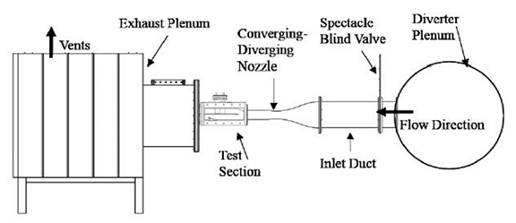Figure 1. Schematic diagram of the wind tunnel facility

Figure 2 displays the test section for the current study. The test section is constructed with a flat bottom wall, a diverging top wall, and two side walls. The test section contains a shock-wave-holding plate and a choking flap.

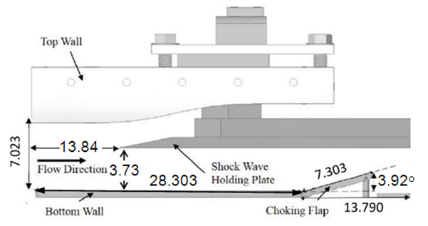Figure 2. Schematic diagram of test section. All dimensions are given in cm

The angle of the choking flap, as well as the normal and streamwise positions of the shock-wave-holding plate, are adjustable. For the present study, the shock-wave-holding plate is parallel to the bottom wall, 13.84 centimeters downstream of the test section entrance, and 3.73 centimeters from the bottom of the test section. The choking flap is set to an angle of 3.92 degrees.

During wind tunnel tests, a shadowgraph system records time-varying, shock-wave flow features within the test section. The system consists of a white-light source (SugarCUBE LED Illuminator model number 66-032, manufactured by Edmond Optics Corp.) and two 152.4-mm-diameter focusing mirrors. The mirrors are aligned such that the light beam is parallel to the spanwise direction of the test section and orthogonal to the side walls. This alignment arrangement provides images with the greatest contrast of density-varying visualized flow features. Varying density variations within the flow field are thus captured within a visualized volume as a line-of-sight integrated image, which covers most of the span of the test section. This approach is employed to illustrate three-dimensional flow variations which are present. Note that the second 152.4-mm-diameter focusing mirror additionally focuses the resulting shadowgraph image into the AF Micro NIKKOR 200 mm 1:4D ED camera lens, which is connected to a Phantom v711 high speed camera, which is manufactured by the Ametek Materials Analysis Division of Vision Research Company.

2.2. Overall Data Acquisition and Analysis Procedures

Phantom Camera Control 2.7 software is employed to process the images which are captured by the Phantom camera. Spatial resolution of each image is 20 micrometers per pixel location. The exposure time is 1.0 μs at all sampling rates which are employed within the present investigation. Digitized shadowgraph visualization images are acquired at a data acquisition rate 10 kHz. Additional data analysis and processing are accomplished using MATLAB version R2019b software. Associated programs are used to track shock wave position variations with time and to quantify grey scale pixel intensity variations with time in flow areas of interest. These analysis steps are followed by calculations to determine distributions of power spectral density (PSD) and magnitude squared coherence (MSC) as they vary with frequency.

Ligrani et al. [12] provide additional information on the facility, test section, and data acquisition procedures.

2.3. Power Spectral Density Determination

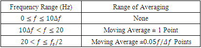
The first step in the determination of distributions of power spectral density (PSD) with frequency is the application of a 5^th order Butterworth filter which attenuates all frequencies above 90 percent of the Nyquist folding frequency. This is accomplished using the butter command within MATLAB version R2019b software. The next step is the application of Welch’s method using the pwelch command within MATLAB to obtain PSD distributions. Each distribution is determined with eight segments and a 50 percent overlapping Hanning data window. The following equation shows how the length of the Hanning window L_s is calculated. Within this equation, L is the total number of measurements and N is the number of window segments.

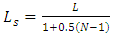(1)

Within the present investigation, L_s is rounded down to the nearest integer. As Welch’s method is implemented, the Fast Fourier Transform (FFT) routine converts time domain data into frequency domain data. This approach gives one spectrum for each Hanning window. These are then ensemble averaged together to provide a single spectrum. This result is subsequently truncated from 0 Hz to the Nyquist folding frequency value.

The magnitude of the PSD or P_xx is calculated using the following equation in which Y(f) is the frequency domain data value, f_s is the sampling frequency, and S is a normalization factor for the Hanning window.

(2)

The resulting P_xx frequency resolution Δf is then given by

(3)

where f_s is the sampling frequency and L_s is the number of data points. Note that PSD values are determined relative to pixel value variations with time.

2.4. Magnitude Squared Coherence Determination

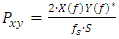
Magnitude squared coherence (MSC) correlation analysis is used to provide information of flow phenomena which are interacting with each other in a coherent manner at different frequencies. The MSC determined value C_xy quantifies the correlation between two datasets, from 0 to 1, as a function of frequency. This analysis is performed using MATLAB with the mscohere function. With this approach, MSC is expressed using an equation of the form

(4)

where P_xx is the PSD of the first signal, P_yy is the PSD of the second signal, and P_xy is the cross power spectral density (CPSD) between the two signals. The CPSD value P_xy is determined using the equation which is given by

(5)

where X(f) is the frequency domain signal for the first dataset, Y(f)* is the complex conjugate of the frequency spectrum for signal two, f_s is the sampling frequency, and S is a normalization factor for the Hanning window.

Data produced by MSC analysis are occasionally very noisy, with greater data scatter as the frequency gets higher. A moving average is utilized to remedy this issue. The equations employed to determine the associated average values are shown in Table 1. From this information, it is apparent that the number of points averaged varies with frequency within the smoothing algorithm.

Table 1. Magnitude squared coherence MSC data moving averaging arrangements

3. Statistical Analysis Results

Within the present investigation, magnitude squared coherence and power spectral density variations with frequency are determined from instantaneous gray scale variations determined from two statistical analysis approaches: tracked instantaneous shock wave motions and from groupings of stationary pixel locations. The tracking approach provides data which are more physically representative of unsteady flow physics. This is because grayscale pixel intensity variations from stationary locations are affected by a shock wave only as it traverses this fixed location. Resulting data then only represent transient and intermittent motion of the shock wave rather than complete unsteady shock wave motion.

3.1. Shock Wave Tracking Determination and Results

Shock wave instantaneous locations are tracked along horizontal lines that cross the shock wave. These line placements are solid black and are shown in Figure 3. When the normal shock wave is tracked, the line is located 0.68 cm below the shock-wave-holding plate. When the lambda foot rearward oblique shock wave is tracked, the line is located 2.54 cm below the shock-wave-holding plate. Overall, Figure 3 presents an instantaneous shadowgraph image for one individual digital frame showing different flow phenomena within the test section. Open white squares within this figure denote locations used for stationary analysis using 5 by 5 pixel arrays.

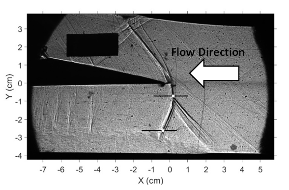Figure 3. Instantaneous shadowgraph image for one individual digital frame showing different flow phenomena within the test section. Solid black horizontal lines denote locations employed for shock wave tracking. Open white squares denote locations used for stationary analysis using 5 by 5 pixel arrays. Flow direction is from right to left

Figure 4 shows the pixel intensity gray scale value variation with streamwise pixel location across the normal shock wave for a location 0.68 cm below the shock wave holding plate. Data are given for three different frame numbers which correspond to three different points in time. As such, each data set within this figure represents values as they vary spatially at one instant in time. Arrows denote data values used to indicate shock wave locations. The position of the normal shock wave along the line is thus determined at the pixel value with the lowest grey scale. This method is appropriate since shock waves produce extreme local density changes and because shadowgraph visualizations show changes resulting from variations of the second derivative of the fluid density. The same pixel intensity gray scale value variation data in Figure 4 are again presented in Figure 5, but as dependent upon dimensional streamwise location. The associated conversion of values along the horizontal scale in these two figures is based upon the 10 kHz sampling frequency. Portions of the data in Figures 4 and 5 evidence considerable flow unsteadiness. However, the low pixel value which identifies the instantaneous shock wave position is outside the range of this unsteadiness and is therefore a definitive indicator of instantaneous shock wave position.

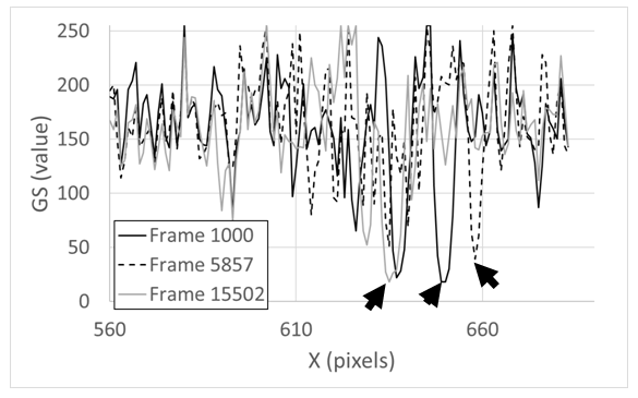
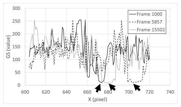Figure 4. Pixel intensity gray scale value variation with streamwise pixel location across the normal shock wave for a location 0.68 cm below the shock wave holding plate. Data are given for different frame numbers which correspond to different points in time. Arrows denote data values used to indicate shock wave locations

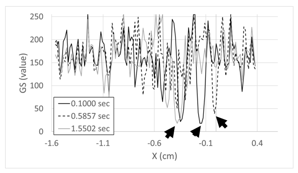
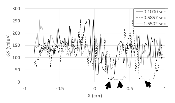Figure 5. Pixel intensity gray scale value variation with dimensional streamwise location across the normal shock wave for a location 0.68 cm below the shock wave holding plate. Data are given for different points in time. Arrows denote data values used to indicate shock wave locations

Similar results are provided in Figures 6 and 7 for tracked locations of the lambda foot rearward oblique shock wave. Here, local flow unsteadiness relative to the oblique shock wave is even more pronounced than in the previous two figures. However, as for the normal shock wave, the instantaneous position of the oblique shock wave is definitively indicated by minimum pixel values which are generally outside the range of the flow unsteadiness which is present prior and after this event.

Figure 6. Pixel intensity gray scale value variation with streamwise pixel location across the lambda foot rearward oblique shock wave for a location 2.54 cm below the shock wave holding plate. Data are given for different frame numbers which correspond to different points in time. Arrows denote data values used to indicate shock wave locations

Figure 7. Pixel intensity gray scale value variation with dimensional streamwise location across the lambda foot rearward oblique shock wave for a location 2.54 cm below the shock wave holding plate. Data are given for different points in time. Arrows denote data values used to indicate shock wave locations

To determine shock wave position with respect to time, relative to data such as are presented in Figures 4, 5, 6, and 7, MATLAB program coding is employed to determine the grey scale pixel intensity across the shock wave for every shadowgraph digitized image. Next, the pixel which presents the minimum for every digitized image is determined, which is then converted to a dimensional spatial value. An example of the resulting shock wave position variation with time is shown in Figure 8. Here, X’ is the streamwise shock wave position, such that X’ equals zero at the average position of the shock wave. Within this figure, times corresponding to data in Figs. 3 and 4 are annotated with grey arrows. Figure 8 illustrates unsteady normal shock wave motion, including several intervals with increased flow unsteadiness which start around t equals 0.4 secs. and around t equals 0.52 secs.

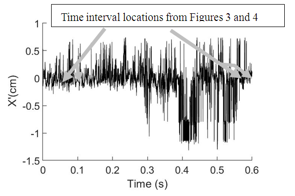Figure 8. Normal shock wave dimensional streamwise location variation with time for a location 0.68 cm below the shock wave holding plate. Data are obtained from Figures 4 and 5 with associated data intervals denoted by gray arrows

3.2. Power Spectral Density Results

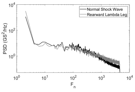
Power spectral density (PSD) distributions provide estimates of the amount of energy associated with each frequency of the unsteady behavior. Figure 9 shows power spectral density variations with frequency based upon tracked locations of the normal shock wave and the lambda foot rearward oblique shock wave. Overall qualitative variations of the PSD distributions for both the normal shock wave and the rearward lambda shock wave leg have similar shapes, with aligned peaks at 8.5 Hz, 16 Hz, and 25 Hz. In addition, both data sets show a negative slope which indicates a higher energy content associated with larger length scales and lower frequencies. The most important difference between these two data sets in Figure 9 is different quantitative magnitudes at each frequency, with consistently higher values associated with the normal shock wave.

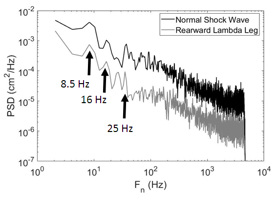Figure 9. Power spectral density variations with frequency based upon tracked locations of the normal shock wave and the lambda foot rearward oblique shock wave

For comparison, PSD analysis is also performed using time variations of grey scale pixel intensity which are ensemble averaged within a 5 by 5 arrangement of stationary pixels. The locations of these 5 by 5 arrays are denoted within Figure 3 as white squares. Figure 10 shows the resulting power spectral density variations with frequency for stationary pixel locations in the vicinity of the normal shock wave and in the vicinity of the lambda foot rearward oblique shock wave. Decreasing magnitudes with frequency are evident for both distributions, with similar quantitative magnitudes. However, note that these distributions lack the prominent aligned peaks and troughs that are evident within Figure 9. This means that physically relevant unsteady flow information is missing from data presented within Figure 10.

Figure 10. Power spectral density variations with frequency based upon stationary pixel locations in the vicinity of the normal shock wave and in the vicinity of the lambda foot rearward oblique shock wave

3.3. Magnitude Squared Coherence Results

Figure 11 presents magnitude squared coherence variations with frequency based upon three different analysis approaches, methods 1, 2, and 3. Method 1 is based upon time variations of grey scale pixel intensity value variations within a 5 by 5 pixel region in the vicinity of the normal shock wave and within a 5 by 5 pixel region in the vicinity of the lambda foot rearward oblique shock wave. Method 2 is based upon the tracked time varying position of the normal shock wave and grey scale pixel intensity value variations within a 5 by 5 pixel region in the vicinity of the lambda foot rearward oblique shock wave. Method 3 is based upon tracked locations of both the normal shock wave and the lambda foot rearward oblique shock wave. Within Figure 3, the locations used for stationary analysis with the 5 by 5 pixel arrays are denoted using open white squares. Line locations used for tracking shock wave locations are also shown in Figure 3.

The highest coherence values within Figure 11 are produced using method 3. Local maxima peaks for this method are located at 8.5 Hz, 16 Hz, and 25 Hz, which correspond to similar PSD peaks in Figure 9. Within Figure 11, a similar peak at 8.5 Hz is present which is associated with methods 1 and 2, and a peak at 25 Hz is associated with method 2. There is also a very small peak for Method 1 around 35 Hz, whereas with Method 3, a large local maximum is present near the same frequency. This locally high value with method 1 is not present when methods 2 and 3 are employed. This is partially due to methodology for methods 2 and 3 because correlations are determined for spatially tracked streamwise position data relative to an average value which is set equal to zero. This zero value also appears in correlation distributions for frequencies near 0 Hz due to the associated Fourier transform offset. However, this is not the case for method 1 results. The superficially high MSC values at low frequencies for the method 1 results are additionally due to the intermittent motion of the shock waves as they transverse stationary pixel locations.

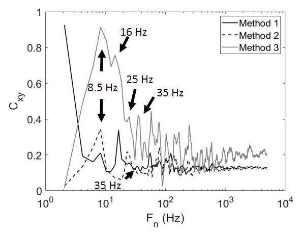Figure 11. Magnitude squared coherence variations with frequency based upon three different analysis approaches, methods 1, 2, and 3, where method 3 is based upon tracked locations of the normal shock wave and the lambda foot rearward oblique shock wave

The overall conclusion from these trends, especially the highest correlation values at most frequencies with method 3, is that flow phenomena associated with tracked positions of the normal and oblique shock waves are highly correlated with each other, which means that method 3 provides the most physically relevant results. Figure 11 thus provides insight regarding the relevance of other methods of data extraction compared to tracking spatial variations of shock wave position with time. While methods 1 and 2 show local maxima at the same frequencies as results obtained using method 3, quantitative magnitudes of peak values associated with methods 1 and 2 are less than with method 3, indicating lower ability to capture and quantify physical phenomena within the flow.

4. Summary and Conclusions

Of the different statistical analysis approaches used for magnitude squared coherence determination, method 3, wherein analysis is based upon tracked locations of both the normal shock wave and the lambda foot rearward oblique shock wave, provides the most physically relevant results. This relevancy is demonstrated by the highest coherence values for all frequencies which are provided using method 3, relative to methods 1 and 2. When magnitude squared coherence values are based on grayscale variations from flow phenomena determined at fixed pixel locations, anomalous coherence values are produced due to inappropriate analysis methodologies and because of intermittent motion of the shock waves as they transverse stationary pixel locations.

Power spectral density quantitative and qualitative data trends lead to similar conclusions. Illustration is provided by power spectral density variations with frequency which are based upon tracked locations of the normal shock wave and the lambda foot rearward oblique shock wave. Ensemble averaged spectra for these two types of tracked shock waves have peaks which are aligned with each other at frequencies of 8.5 Hz, 16 Hz, and 25 Hz. These peaks are also in excellent agreement with frequencies of local maxima within magnitude squared coherence distributions which are based upon tracked shock wave location analysis.

ACKNOWLEDGEMENTS

The present research effort was funded by the CBET Thermal Transport Processes Program, National Science Foundation, Award Number 2041618.