1. Introduction

In this article we propose a simple and effective procedure for the construction of socioeconomic status indices using principal component analysis. This type of index has aroused great interest in recent years, mainly for use in public policy design. It allows ranking and spatializing the socioeconomic status of a given locality, municipality, state, region or even an entire country. Once the socioeconomic status is ranked and spatialized, policies can be designed to target specific groups of individuals.

Although the method we propose can be used to build other types of composite indices, the focus of this article is on the construction of socioeconomic status indices. According to [1], “socioeconomic status is the social standing or class of an individual or group. It is often measured as a combination of education, income and occupation” and “examinations of socioeconomic status often reveal inequities in access to resources, plus issues related to privilege, power and control”.

According to the above definition, the socioeconomic status of individuals involves multiple dimensions. This characteristic allows the creation of different socioeconomic status indices, with specific purposes, in addition to the possibility of using different methods to construct them. Regarding these indices, [2] discuss what they are, what they are for and how they are constructed. [3], in turn, review different methods used to build socioeconomic status indices.

Regardless of the method used to build composite indices, it is important to consider issues related to choosing variables, preparing data or problems such as data clustering. However, the methods used in the construction of these indices in which the choice of the weights of the variables or sub-indices is made subjectively are subject to strong criticism. The principal component analysis method is not subject to this type of criticism. In fact, when applying this method, the weights of the variables or sub-indices emerge naturally. This feature and the ease of working with multiple variables has contributed to the increasing use of principal component analysis in the construction of composite indices.

Composite indices that are constructed using principal component analysis are based on principal components drawn from the sample of variables, with each principal component being a linear combination of the original variables. Most authors who use principal component analysis to build socioeconomic status indices consider only the first principal component and its relationship to the original variables as a composite index (see, for example, [4] or [5]). Others consider only the first two principal components, but interpret them as two distinct composite indices. This is the case, for example, of [6], who developed the Institut National de Santé Publique du Québec (INSPQ) index; in their work, the first principal component comprises the weights of a “material-based” deprivation index and the second principal component comprises the weights of a “social-based” deprivation index.

The purpose of this article is twofold: first, to propose the construction of socioeconomic status indices using principal component analysis that consider not only the first principal component, but a weighted average of the first principal components. As mentioned earlier, current literature on socioeconomic status indices generally considers only the first principal component as a composite index; and second, to illustrate the proposed method with the calculation of a social vulnerability index for the municipalities of an area of the São Francisco river basin, Brazil, using data from the demographic census.

We give the following reasons to justify constructing a socioeconomic status index as a weighted average of more than one principal component: i) in general, the first principal component explains only a small part of the variance of the original data. A composite index with more than one principal component would explain a greater portion of the variance of the original data; ii) the socioeconomic status of individuals involves multiple dimensions and hardly a single principal component could capture all these multiple dimensions.

2. Principal Components and Socioeconomic Status Indices

Principal component analysis is a statistical method that transforms a set of correlated variables into another set of uncorrelated variables called principal components (for more details on this method, see, for example, [7], [8], or [9]). These principal components are linear combinations of the original variables and must satisfy certain properties. In this transformation, information on data variability is preserved and their complexity is reduced. To obtain the principal components, the variance-covariance matrix or correlation matrix of a sample of random variables is used.

Formally, suppose the vector represents a set of n random variables with mean and variance-covariance matrix . Let be the random vector of the corresponding standardized variables, that is,

where represents the variance of variable Note that the covariance between variables and is related to the covariance between variables and as follows

that is, the variance-covariance matrix of z corresponds to the correlation matrix of x. In this article, the correlation matrix of x will be denoted by C.

Although the principal components can be obtained from the variance-covariance matrix of x or the correlation matrix of x, they are not necessarily the same. This implies that the interpretation of the results must take into account the choice of the matrix that will be used to extract the principal components. [10] recommend using the correlation matrix to extract principal components when the scales of variables vary widely or they have very different variances. In this article, the analysis will be carried out with the correlation matrix, since the variables generally used to obtain socioeconomic status indices are diverse and with very different variances.

In this sense, the principal components are associated with the random vector z, such that

where are constants that satisfy certain conditions. It can be shown that the mean of is equal to zero, , and its variance is given by where

The principal components are obtained sequentially: first, is selected to capture as much of the variation in the original data as possible amongst all linear combinations of z such that Then is selected to account for a maximum proportion of the remaining variance subject to not being correlated with the first principal component, and Subsequent principal components are obtained in a similar manner. Formally, the jth principal component is the linear combination that has the greatest variance subject to the following conditions

As it is an optimization problem with equality constraints, the Lagrange method can be used to obtain the solution (see, for example, [7]). The results of applying this method show that the vector of coefficients that defines the jth principal component, is the eigenvector of the matrix C associated with its jth largest eigenvalue. Let be the n eigenvalues of C. It can be shown that that is, the variance of the jth principal component is equal to the eigenvalue . It can also be shown that Thus, the proportion of the total variance of the standardized variables explained by the jth principal component is given by

and the percentage of the total variance explained by the m first principal components, is given by

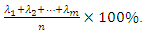According to [11], “applied principal component analysis consists most often of a mere computation of eigenvectors and eigenvalues of a sample covariance matrix or correlation matrix” (p. 606). That’s largely what we are going to do in this article. To start, we summarize the main results of the principal component analysis related to eigenvalues and eigenvectors that will be useful for the construction of socioeconomic status indices in the following properties:

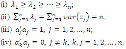As mentioned in the introduction, some authors consider only the first principal component, as a socioeconomic status index and others consider the first two main components, and , but as two distinct indices. In this article we propose the construction of a socioeconomic status index as a weighted average of the first m, principal components. The idea behind this proposal is that the first few principal components will represent a substantial proportion of the variation in the original variables and can therefore be used to provide a convenient lower-dimensional summary of these variables.

In this sense, we can construct a socioeconomic status index (SSI) as a linear combination of all the principal components as follows

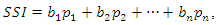where the weight vector, with is given by

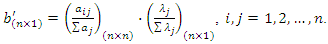(1)

Note that the only information needed to construct the socioeconomic status index indicated above are the scores of the principal components and the values of the eigenvalues and eigenvectors obtained from the sample of random variables. From a practical point of view, it is usual to consider the first few principal components as long as they satisfy some criterion. In practical applications in the area of social sciences and humanities, [8] suggests choosing the first principal components until reaching at least 60% of the total variation of the original data. Assume that the first principal components satisfy the criterion of [8], then the socioeconomic status index is given by

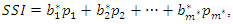where represents the vector of corrected weights, such that Note that if we were to use the original weights we would have a result whose sum of weights is not equal to 1. To correct the weights, we use the following expression:

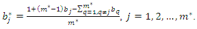This correction of the weights is fundamental to obtain a socioeconomic status index as a weighted average of the first principal components. To illustrate this correction of weights, suppose that the first three principal components were selected to construct a socioeconomic status index and that the original weights are and . Applying the correction formula, knowing that , we have

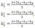Note that, after correction, we have . It is important to keep in mind that this procedure for constructing a socioeconomic status index must take into account all variables and all observations of each variable. Suppose you want to build a socioeconomic status index from a sample of 10 variables 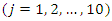and each variable contains 100 observations 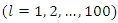. In this case, the principal components of each observation are calculated, that is,

where represents the jth principal component of the lth observation. After calculating the 10 principal components associated with each to the 100 observations, the weights corresponding to the sample of variables can be obtained (see expression for determining the vector of weights b above). Suppose further that three principal components were selected to build the socioeconomic status index. In this case, this index is constructed for each observation of the sample of variables as follows:

where represents the corrected weight, and denotes the principal component j associated with observation l of the sample of variables. After carrying out all the calculations, one obtains, as a result, an interval composed of 100 socioeconomic status indices (one index for each observation of the sample of variables) that can divided equally or using some other criterion to form the socioeconomic status classes (levels). This number of classes is defined according to the purpose of the study or to meet public policy interests. Commonly used arbitrary cut-off points classify the lowest 40% of individuals as 'poor', the highest 20% as 'rich' and the remainder as the 'average' group (see, for example, [12]).

To avoid an eventual negative component in the weight vector, b, another possibility to define weights is to use the expression (2) given in the following proposition

Proposition. If the correlation matrix is positive definite and the eigenvectors associated with C are such that , and , , then the weight vector b given by

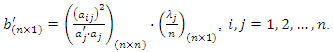(2)

satisfies the properties and

Proof. From the expression , we have , , and the eigenvalues are given by Substituting the expression for in (2), we have Since is arbitrary, the proof is complete.

If we use expression (2) to define the weight vector b, no correction is needed if , where is the number of principal components used to build the composite index. In this case,

Standard statistical software (such as STATA or SPSS) can be used to perform the necessary calculations and build composite indices. In the illustration of the use of the proposed method in the next section, the statistical analysis was performed with the R software ([13]) and ArcGis® ([14]) was used to spatialize the results (vulnerability classes) of the study area.

3. Results: Social Vulnerability Index

This section presents the calculation of a social vulnerability index for the municipalities of an area of the São Francisco River Basin as un illustration of the method proposed in this article. This basin has a drainage area of about 630 thousand square kilometers and includes 521 municipalities belonging to six different states (Minas Gerais, Goiás, Bahia, Pernambuco, Alagoas e Sergipe) plus the Federal District. The basin has a population of over 16 million inhabitants, with a large part of it, around 77% of the total, inhabiting urban areas. The São Francisco River is often called the “river of national integration” because it unites different physiographic regions of the country, especially the Southeast and Northeast.

Due to its large extension and diversity, the São Francisco River Basin is divided into Upper, Middle, Sub-medium and Lower São Francisco. According to [15], taking 2014 as a reference, the shares of these regions in the Gross Domestic Product (GDP) of the basin are as follows: Upper São Francisco (86.6%), Middle São Francisco (4.9%), Sub-medium São Francisco (5.4%) and Lower São Francisco (3.1%). This distribution of GDP in the basin highlights the economic discrepancy between these regions, showing that most of the wealth is generated in the Upper São Francisco.

To calculate the social vulnerability index, we considered only part of the Upper São Francisco region. This study area is equal to 58,204.65 square kilometers and comprises 105 municipalities. Figure1 locates the São Francisco River basin in Brazil and also shows this study area. The São Francisco River originates in this selected area, more specifically in Serra da Canastra, in the central-western part of the state of Minas Gerais. This is a predominantly urban area and is home to various economic activities, such as steel production, mining, textile industry, chemical industry and industrial equipment.

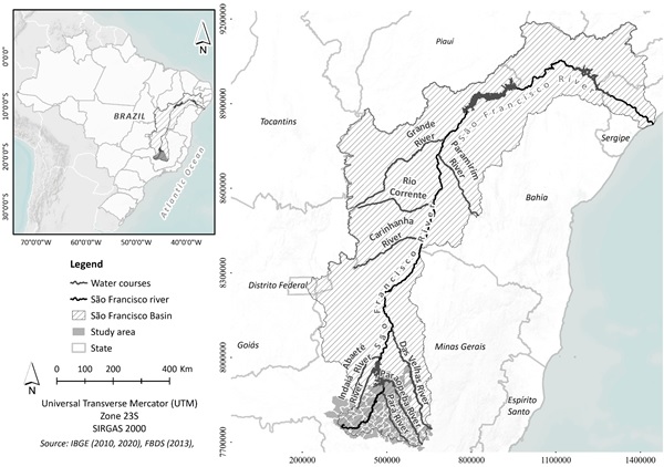Figure 1. São Francisco River basin and study area

To calculate the social vulnerability index, we selected 12 variables from the last demographic census ([16]). This selection of variables took into account the international literature and, in the Brazilian context, the work of [17]. These variables were classified into three categories: human capital, urban infrastructure and occupation/income and are listed below.

Human capital

• % of illiterate children from five to 14 years old

• % of illiterate female heads of households

• % of people aged 15 and above

• Infant mortality (per 1,000 live births)

Urban infrastructure

• % of dwellings with inadequate sewage disposal systems

• % of dwellings without access to the general supply water network

• % of families with an income of less than one minimum wage and with inadequate housing conditions

• % of dwellings without access to the general electricity grid

Occupation/income

• % of people earning up to minimum wage

• % of responsible people with no monthly nominal income

• % of people without incomes of their own

• % of families that depend on the income of older adults

All variables are in percentages, except infant mortality. The percentages were obtained by dividing the value of each variable in the municipality by the population of the respective municipality. Note that for the calculation of the social vulnerability index we have 12 variables and 105 observations for each variable. After preparing the data, the principal component analysis was carried out, first obtaining the correlation matrix of the variables. From the principal components extracted from the correlation matrix, we selected the first four that explain 70.89% of the variance of the original data and we used expression (2) to define the vector of weights in the construction of the social vulnerability index.

The values of the social vulnerability index obtained from the sample of variables ranged from a minimum of 0.05244 (Belo Horizonte) to a maximum of 0.313853 (Piedade dos Gerais). We divided the range of variation of this social vulnerability index equally into three classes, with break values equal to 0.140, 0.227 and 0.314. These vulnerability classes (or levels) were called “low” (variation from 0.052 to 0.140), “moderate” (variation from 0.141 to 0.227), and “high” (0.228 to 0.314). The vulnerability results obtained for these different classes were spatialized for better visualization (see Figure 2).

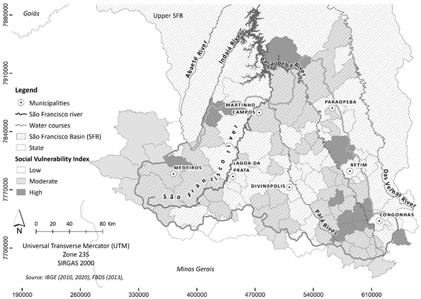Figure 2. Social vulnerability for the municipalities of an area of the São Francisco River basin

The municipalities classified as less socially vulnerable, according to our classification, are Belo Horizonte, Itaúna, Contagem, Nova Serrana, Pará de Minas and Sete Lagoas. On the other hand, the municipalities classified as the most vulnerable in the study area are Piedade dos Gerais, Itaverava, Rio Manso, Esmeraldas, Moeda, Desterro de Entre Rios, Felixlândia, Jeceaba, Quartel Geral and Serra da Saudade. The other municipalities in the study area belong to the moderate class of social vulnerability. Note that only ten municipalities out of the 105 considered in our study (9.52%) were classified as the most socially vulnerable. This result is consistent with the socioeconomic information available for the São Francisco River basin, especially those for the Upper São Francisco region.

Once the social vulnerability of a given area or region is ranked and spatialized, public policies can be designed to target (directly or indirectly) specific groups of individuals. Another alternative way of using this type of information is to design differentiated policies considering simultaneously different groups of individuals. In this case, considering more than three classes of social vulnerability would allow a more detailed and accurate ranking.

4. Conclusions

In this article we present a simple and effective method for building socioeconomic status indices based on principal component analysis. The index is calculated as a weighted average of principal components selected from among those extracted from the correlation matrix of a sample of random variables. The calculation of a social vulnerability index for municipalities in an area of the São Francisco river basin, Brazil, using data from the demographic census was used to illustrate the method.

The proposed method is sufficiently general and can be applied to obtain other types of composite indices and not just socioeconomic status indices. As the index obtained by the principal components analysis is based on a set of random variables, the choice of these variables is fundamental to obtain a reliable and useful index to meet the objectives that motivated its construction. In this sense, the set of selected variables must be sufficient to represent with some accuracy the indicator being measured, such as the socioeconomic status of individuals. In most cases, it is also necessary to prepare the data or do some transformation of variables before obtaining the correlation matrix. [18] discuss these and other issues associated with the construction of indices using principal component analysis.

Finally, although the presentation of the proposed method was based on the correlation matrix to extract the principal components, the same procedure can be done considering the covariance-variance matrix of the original data. In this case, it is convenient that the variances of the original variables are close to each other. It is also possible to use other criteria for the selection of the first principal components in the construction of the composite index and not just the criterion presented in this article.