Enesi Latifat O.1, Turkur D.2, Dikko H. G.1
1Department of Statistics, Ahmadu Bello University, Zaria
2Department of Community Medicine, Ahmadu Bello University, Zaria
Correspondence to: Enesi Latifat O., Department of Statistics, Ahmadu Bello University, Zaria.
| Email: |  |
Copyright © 2022 The Author(s). Published by Scientific & Academic Publishing.
This work is licensed under the Creative Commons Attribution International License (CC BY).
http://creativecommons.org/licenses/by/4.0/

Abstract
In this work, Survival analysis of neonatal jaundice patients using Accelerated Failure Time(AFT) Model was carried out. The parametric estimates of the model were derived using maximum likelihood method. Furthermore, we applied the parametric model to a secondary data of 150 neonatal jaundice patients collected from Ahmadu Bello University Teaching Hospital, Shika, Zaria. The Predictive models that could be used to predict the survival times of neonatal jaundice patients were formulated. The data was analysed using R statistical software to estimate the parameters. Kaplan Meier (KM) curves were plotted for the seven categorical variables with time recorded in days indicated that patients who use tradition medicine have a higher survival time than patients who employed orthodox. Patients who do not visit Antenatal care have shorter survival time than those who used the Antenatal care. The results for the GWL AFT model shows that the survival time of neonates increased statistically and significantly because they were influenced by Antenatal visit, weight, type of delivery and gender respectively. The parametric model of the Generalized Lindley-Weibull (GLW) model performed better when compared with the results of some common existing parametric survival models based on the performance measures.
Keywords:
Generalized Lindley-Weibull (GLW), Kaplan Meier, Neonatal jaundice
Cite this paper: Enesi Latifat O., Turkur D., Dikko H. G., Survival Analysis of Neonatal Jaundice Patients in Ahmadu Bello University Teaching Hospital, Shika Zaria, International Journal of Statistics and Applications, Vol. 12 No. 3, 2022, pp. 55-62. doi: 10.5923/j.statistics.20221203.01.
1. Introduction
One of the features of survival data structure is censoring. Survival data are generally collected for a time interval in which the occurrences of a specific event are obtained. Survival data modelling has plays a vital roles in the application of statistics in epidemiology [2], thus, survival analysis of neonatal jaundice patient was carried out to model time to surviving neonatal jaundice. In survival analysis, censoring is the loss of observation on the lifetime variable of interest in the middle of the study due to various reasons. For most censoring types, a section of survival time for censored observations are observable and can be utilized in calculating the risk of experiencing a particular event. Censoring is generally divided into several types, such as right, left and interval censoring. Right censoring is the type of censoring that occurred when an individual has entered a study but is lost to follow-up, the actual event time is placed somewhere to the right of the censored time along the time axis [13]. As right censoring occurs more frequent than other types and its information cannot be excluded in the estimation of a survival model. Left censoring can occur when an individual failed before data collection began. Interval censoring occurs when an individual requires follow-ups or inspections. The interval is, begin at zero or end at infinity.Cox Proportional Hazard model is also referred to as semi-parametric model. It makes assumption about parametric form for the effect of the predictors on the hazard but no assumptions about non-parametric model being make. The interpretation of Cox proportional or Cox regression model means that the effects of different variables on survival are constant over time. One of the basic assumptions in a Cox regression model is the proportional hazard assumption, since it does not assume any form of distribution for survival times [3]. Proportional hazard simply means that the ratio of the hazards for two subjects, say, O and P at time t is the same for all values of t. Also, if the assumption of proportional hazards is true for two groups of survival times, say Group O and Group P, then the true survivor functions for the two groups fail to cross each other then we say they are parallel which is necessary but not a sufficient condition for proportional hazards. In modeling with explanatory variables, assumption of proportional hazards means that the effects of the different variables on survival are constant over time [7].Parametric model can be estimated either by the proportional hazard or the Accelerated Failure Time (AFT) regression model. In this study, we will adopt AFT Model. The AFT model describes a situation where the mechanical or biological life history of an event is accelerated (or decelerated). One advantage of using the specification of AFT regression model is that it covers a wide scope of the survival time distribution [13]. AFT Model is a general model for data consisting of survival times, in which explanatory variables measured on an individual are assumed to act multiplicatively on the time dependent, and so affect the rate at which an individual proceeds along the time axis. Consequently, the model can be interpreted in terms of the speed of progression of a disease, for example, those receiving treatment say, A and those receiving treatment say, B, This model assumes that the survival time of an individual on one treatment is a multiple of the survival time on the other treatment; as a result, the probability that an individual on treatment A survives beyond time t is the probability that an individual on treatment B survives beyond time [5].An important feature of the new families of generalized distributions is based on their flexibility and compatibility to analysed real life data [2]. Over the period, Generalized Webull-Lindley (GLW) distribution has been developed by many researcher to model survival data such as [6], [12], their study GLW appeared to be more flexible when compared with other distribution. Jaundice is the most common disease in infants within the first week of life and it causes an infant mortality if not diagnosed and treated on time. The preventable factors that cause the readmission of the infant after birth is very important. This inspires the study of survival of neonatal jaundice with possibly time dependent covariates. Therefore, we are looking for the best AFT model to predict the most common factors rising neonatal jaundice. And there is also need to develop the Generalized Lindley-weibull Survival Model in order to investigate some associated factors to the survival time of the neonatal jaundice patients.
2. Materials and Methods
The survival analysis of time to event data however covers a wide scope which involves several parametric distributions as could be possible, but the researcher has narrowed down the study to cover four distributions. For the purpose of this research, application of the AFT models (Exponential, Wiebull, Log-logistics, and Generalized Lindely -Weibull) in analyzing neonatal jaundice data will be discussed.
2.1. Survival Function
The survival function is a probability of an individual surviving longer than a given period of time  [4]. Let T denote a continuous non-negative random variable representing time until some event of interest, with probability density function (pdf) f(t) and cumulative distribution function (cdf) F(t)= Pr{T ≤ t}, the probability of being alive at t. The survival function is given by
  and
and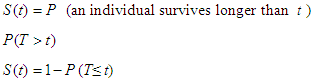 | (1) |
using the definition of cumulative distribution function  of
of  , we can write;
 | (2) |
Here  is a non-increasing function of time t with the following properties. (i) i.e. at the beginning of the study (ii)
 , which means that everyone will eventually experience the event. However, we will also allow the possibility that
  . This corresponds to a situation where there is a non-negative probability of surviving or not experiencing event. For example, if the event of interest is the time from response until the disease relapse and the disease has a cure for some proportion of individuals in the population, then we have
 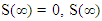 corresponds to the proportion of cured individuals.
2.2. Hazard Function
The hazard function  is also referred to as the conditional mortality rate or instantaneous failure rate or force of mortality. This represents the conditional mortality rate that is, event has not yet occurred [10].
  in terms of cumulative distribution function
  and probability density function
  is given by
 | (3) |
 | (4) |
The hazard function describes the concept of the risk of an outcome (e.g., failure, death) in an interval after time  , conditional on the subject having survived time
  . The hazard functions seems to be more intuitive to use in survival analysis than the pdf because it attempts to quantify the instantaneous risk that an event will take place at time
  given that the subject survived to time
  . A number of models are available for the analysis of the relationship of a set of predictor variables with the survival time.
2.3. Non Parametric Test
2.3.1. Kaplan-Meier Estimate of the Survival Function
Suppose that k individuals have died in a group of individuals. Let 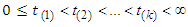 be the observed ordered death times. Let kj be the size of the risk set at
  , where risk set denotes the collection of individuals alive and uncensored just before
  . Let
. Let  be the number of observed deaths at
  . Then the Kaplan-Meier(K-M) estimator of S (t) is given as
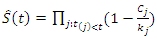 | (5) |
This estimator is a step function that changes values only at the time of each death. In fact, K-M estimator will be shown next to maximize the likelihood in the discrete case.Let  if the ith individual is censored at
  Then, the log likelihood contribution to the total likelihood is
  | (6) |
Then the total log likelihood is given by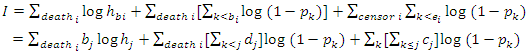 | (7) |
 | (8) |
Where  the number of observed death at is
  is the number censored at
  and
and  is the number of living and uncensored at
  If
If  is the solution of
 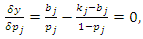 | (3.11) |
then
 (*)This maximizes the likelihood since the total log likelihood function is concave down. So that the K-M estimator of the survival function is
 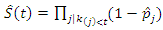 | (9) |
Substitute equation (*) into equation (9), we have | (10) |
Therefore, the K-M estimator is the maximum likelihood estimator. The K-M estimator gives a discrete distribution, if the observations are modelled to come from unknown continuous distribution, the maximum likelihood estimator does not exist [8].
2.4. Cox Proportional Hazards
The Cox Proportional Hazards model is proposed by [3] | (11) |
where  is called the baseline hazard function, which is the hazard function for an individual for whom all the variables included in the model are zero,
  is the values of the vector of explanatory variables for a particular individual, and
  is a vector of regression coefficients. The corresponding survival functions are related as follows:
 | (12) |
This model is known as the Cox regression model, it makes no assumptions about the form of  (non-parametric part of model) but assumes parametric form for the effect of the predictors on the hazard (parametric part of model). The model is therefore referred to as semi-parametric model. The measure of effect is called hazard ratio. The hazard ratio of two individuals with different covariates
  is
is 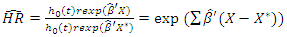 | (13) |
2.5. Accelerated Failure Time Model (AFT)
According to [10], model describes the relationship between a set of covariates and the survival probabilities. For a group with predictor variables or covariates  , where
  represents the time at which individual i experiences a particular event or right censoring
  the AFT model is written mathematically as
 | (14) |
where  is the baseline survival function and
  is an acceleration factor that is, a ratio of survival times corresponding to any fixed value of S(t). The acceleration factor is given according to the formula
 | (15) |
Under AFT model, the covariate effects are assumed to be multiplicative on the time scale and the covariate impacts on survival by a constant factor (acceleration factor).The AFT regression perspective can also be formulated with respect to the random variable T, rather than to logT, for convenience of specifying a likelihood function. | (16) |
 | (17) |
Suppose that Y = log T is linearly associated with the covariate vector x. Then | (18) |
 | (19) |
where  is intercept,
  are the estimates of the covariates
  is scale parameter and,
  is a random variable, T is the random variable assumed to have a particular distribution with survival function S, cumulative density function (cdf) F, and probability distribution function (pdf) f. where
  has the hazard function
  and is independent of
  . Given the equation T ≥ t, the survival function for the ith individual can be mathematically expressed by
 | (20) |
the term  is independent of the disturbance parameter, the survival function S (t) can be written by two separate components;
 | (21) |
Now, | (22) |
 | (23) |
 | (24) |
Comparing equation 21 and 24. We have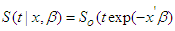 | (25) |
According to the relationship of survival function as  and the hazard function can be expressed in terms of probability distribution function (pdf) and survival function S(t) as follows
 | (26) |
 | (27) |
 | (28) |
Let  and
and  , thus
 | (29) |
 | (30) |
 | (31) |
2.5.1. Generalised Weibull-Lindely (GWL) Model
Let the random variable X follow Lindley distribution with parameter β, the probability distribution function (pdf) and cumulative density function (cdf) of Generalized Weibull–Lindley (GWL) Distribution are given as follows: | (32) |
For 
 | (33) |
Survival function for GWL distribution is given as | (34) |
In terms of the survival model, the GWL hazard function can be formulated as an inverse given by | (35) |
From the equation (35), we have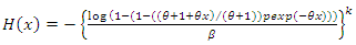 | (36) |
We will consider Weibull model, Log-logistic model, Generalized Weibull-Lindely and Exponential model. For the purpose of comparison, Akaike Information Criterion (AIC) will be used to determine the most appropriate model for the data. The AIC [1], is given by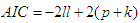 | (37) |
Where ll is the log-likelihood (the probability of the data in a given model), p is the number of parameters/covariates, k = 1 for exponential model and k = 2 for Weibull and Log-logistic model [11]. Smaller AIC indicates better likelihood.
3. Results
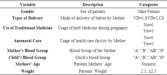
The study aimed at identifying factors that are associated with and are predictive of survival of neonatal jaundice patients. Thus, this chapter contains three sections; the section one describes variables of interest and applies of a non-parametric approach to explain the nature of the variables and how they relate to the survival of neonatal jaundice patients. The second section presents analysis on the PH assumption test for variables and the models. The third section presents the models selection process and the model used for interpretation in this study.Table 1. Variable Description
 |
| |
|
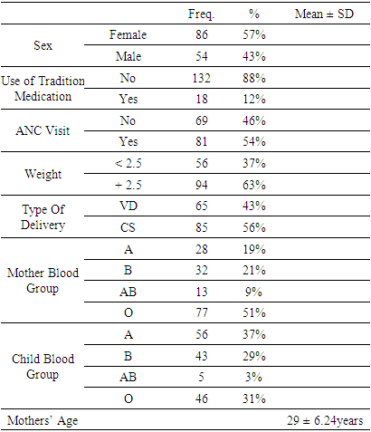
The study used a non-parametric approach to provide a summary of the distribution of the variables. Table 1. Presents description variables and categorization of the covariates for clearer understanding. From table 2, the time to surviving neonatal Jaundice overall median is found to be 45 days, which indicated that 50% of the neonatal patients survived jaundice in less than or equal to 45 days and the other 50% survived jaundice longer than 45 days. This is the survival time at which the cumulative survival function is equal to 0.5. This is summarized in Figure 1.Table 2. Demographic and Medical profile of Mother and Patients (Neonates)
 |
| |
|
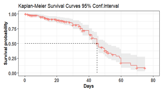 | Figure 1. Survival function of days to survival after the diagnosis of the disease |
The minimum and maximum survival times for neonatal jaundice patients were 0 to 80 days. Eighty days is the predetermined period for which patients who exceeded 80 days after diagnosis are termed to have survived. Figure 1 depicts the Kaplan-Meier probability of the survival of the Neonatal Jaundice patients with a 95% confidence bound, thus the plot observed that the survival probability of the disease decelerate from days 5 above so it is advice that the mother has to be at alert and monitor the child carefully between 0 to 5day of their lives.
4. Discussion
The aim of this research is to identify significant factors that are associated with and are predictor of survival of neonatal jaundice patients. The data used for this study was sourced from Ahmadu Bello University Teaching Hospital, Shika, Zaria. This study used a secondary data collected from the clinic records of 150 Neonatal jaundice patients. The study utilized history of patients or medical records from year 2019 to year 2021. Clinical data such as presentation of the patient, use of traditional medication, birth weight, mother`s blood group, child`s blood group, mode of delivery, and Antenatal Visit Clinic (ANC) visit were collected. Kaplan Meier (K-M) was used to estimate the survival function of neonatal jaundice patients and determine the significant factors associated with the neonatal jaundice disease using the selected parametric distribution.Kaplan Meier (KM) curves are plotted for seven of the categorical variables with time recorded in days. The categorical variables of the study includes Gender, Use of traditional medicine, Use of Antenatal Care, Type of Delivery, Neonates’ Blood group, Mothers’ Blood group and Weight. From table 2, the Kaplan Meier plot for gender, indicated that the female neonates have higher survival probability than male neonates. But with a cautious observation, the curve for the two gender are very close. Though, in the earlier findings, it was revealed that the chances of female neonates have shorter median time of surviving compared to male neonates [6].From Figure 2 it can be observed that patients who used traditional medicine have a higher probability of surviving than patients who did not employ traditional medicine the difference in survival for the two groups runs through the study period. Patients who did not visit Antenatal care have shorter survival time than those who used the Antenatal care. From the plot in Figure 2, the difference in the survival plots for the two groups are quite wide. 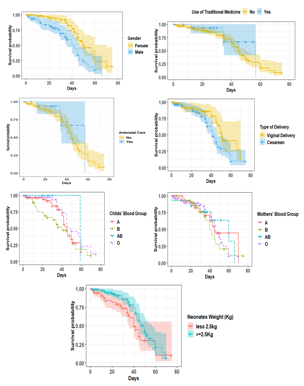 | Figure 2. Survival function of time to survival by covariates |
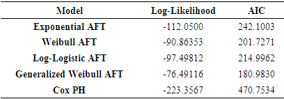
By looking at the child’s blood group in Figure 2, the plot shows that neonates with A blood group has a higher survival probability compared to those with B, AB and O blood group. The difference in survival is visible until after the 70th day where the difference became visible. Considering the neonates’ mothers’ blood group, those with B and AB blood group have higher probability of surviving than other blood group. The survival plots for the groups are quite close suggesting that the differences are not significant enough. This implies that differences between these curves are significant enough. In Figure 2, the plot shows that patients with over 2.5Kg weight have a shorter survival probability than those weighing less than 2.5Kg.In comparing with the Parametric Accelerated Failure Time (AFT) models which are Exponential, Weibull and Log-logistic models, as against the Generalized Weibull Lindley and Cox proportional Hazard model. The models will be compared on the basis of their AIC values to select the best-fitted model and finally the selected model will be used for interpretation. Table 3 presents the hazard ratios for the Semi parametric model (Cox PH), and also the Time Ratio (TR) for the parametric models (Exponential, Weibull and log-logistics and GWL). Generally, AIC is used to select the best models. The lowest AIC leads us to identify the best one. According to the result, all the parametric models had the lowest AIC indicating that they outperform in comparison to Cox PH regression model, and among the parametric models, the Generalized Weibull Lindley (GWL) outperformed the rest of the parametric models by having a lowest AIC of 180.92 as seen on Table 3. Thus, GWL model was considered the best model that fits the data. However, in the studies of [6], [11] GLW appeared to be more flexible when compared with other distribution.Table 3. Cox Regression and parametric Models with prognostic factors
 |
| |
|
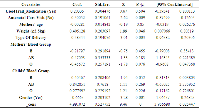
The final results for the GWL AFT model was shown in Table 4 and the result revealed that the survival time of neonates jaundice patients is statistically significantly influenced by Antenatal visit, weight, type of delivery and gender respectively.Table 4. Generalized Weibull Lindley Model
 |
| |
|
5. Conclusions
The Generalized Lindley-weibull (GLW) was studied and applied to neonatal jaundice data. The result of the application based on the performance measures, showed that the Generalized Lindley-weibull (GLW) model is the best fit for modelling neonatal jaundice data. Kaplan Meier (KM) plots for the seven categorical variables with time recorded in days indicated that patients who used traditional medicine will have a higher probability of survival time than patients who did not employ traditional medicine and patients who did not visit Antenatal care will have a shorter survival time than those who used the Antenatal care. The results for the GWL AFT model showed that the survival time of neonates jaundice was statistically significantly influenced by Antenatal visit, weight, type of delivery and gender respectively.
References
| [1] | Akaike H. (1973). “Information Theory and Extension of the Maximum Likelihood Principle “. In B.N. Petrov and F. csaki (eds) 2nd International Symposium on Information Theory, Academia Kiodo, Budapest 267 – 281. |
| [2] | Alzaghal A., Lee C., and Famoye F. (2013). Exponentiated T-X family of distributions with some application. International Journal Probability and statistics. 2, 31-49. |
| [3] | Cox D. (1972). Regression Model and Life-table. Journal of the Royal Statistical Society, 34, 187-220. |
| [4] | Cox D. R. and Oakes D. (1984). Analysis of Survival Data. Chapman and Hall Limited, London. |
| [5] | Everitt B.S. (2002). The Cambridge Dictionary of Statistics. Second Edition. The Edinburgh Building, Cambridge, United Kingdom. |
| [6] | Folorunso S. A. and Osanyintupin O. D. (2018) Comparism of Cox Proportional Hazard model and Accelerated Failure Time Models: An Application to Neonatal Jaundice. International Journal of Public Health and Safety. 3(4) 100-171. |
| [7] | Grover, G., Sreenivas, V., Sudeep K. and Divya S. (2013). Estimation of survival of Liver Cirrhosis Patients, in the presence of prognostic Factors Using Accelerated Failure Time Model as an Alternative to Proportional Hazard Model. International Journal of Statistics and Applications, 3(4), 113-122. |
| [8] | Johansen S. (1978). The product limit estimate as a maximum likelihood estimate. Scandinavian Journal of Statistics 5, 195-199. |
| [9] | Joseph G.C. (2010) Survival analysis: Overview of parametric, nonparametric and semi-parametric approaches and new developments. SAS Global forum, Michigan State University, USA. |
| [10] | Kalbfleisch J.D. and Prentice R.L. (2002). The Statistical Analysis of Failure Time Data. Second Edition. Wiley, New York. |
| [11] | Klein JP, Moeschberger L.M. (2005). Survival Analysis: Techniques for Censored and Truncated Data. Second edition. New York. |
| [12] | Pius M. and Gadde S. R. (2020). Generalized Weibull-Lindley Distribution in modeling Lifetime Data. Journal of Mathematics, 1, 23-38. |
| [13] | Xian Liu (2012). Survival Analysis models and Applications. First Edition, John Wiley & Sons Ltd, The Atrium, Southern Gate, Chichester, United Kingdom. |

 Abstract
 Reference
 Full-Text PDF
 Full-text HTML