-
Paper Information
- Paper Submission
-
Journal Information
- About This Journal
- Editorial Board
- Current Issue
- Archive
- Author Guidelines
- Contact Us
International Journal of Statistics and Applications
p-ISSN: 2168-5193 e-ISSN: 2168-5215
2022; 12(2): 30-41
doi:10.5923/j.statistics.20221202.02
Received: Feb. 12, 2022; Accepted: Mar. 2, 2022; Published: Mar. 15, 2022

Investigating the Persistence of Shocks: Global Warming, Economic Growth and Migration
 Abstract
 Reference
 Full-Text PDF
 Full-text HTML
Erhard Reschenhofer1, Barbara Katharina Reschenhofer2
1Department of Statistics and Operations Research, University of Vienna, Oskar-Morgenstern-Platz 1, Vienna, Austria
2Department of English and American Studies, University of Vienna, Spitalgasse 2-4, Vienna, Austria
Correspondence to: Erhard Reschenhofer, Department of Statistics and Operations Research, University of Vienna, Oskar-Morgenstern-Platz 1, Vienna, Austria.
| Email: |  |
Copyright © 2022 The Author(s). Published by Scientific & Academic Publishing.
This work is licensed under the Creative Commons Attribution International License (CC BY).
http://creativecommons.org/licenses/by/4.0/

Choosing the value of 0.5 for the fractional differencing operator can be helpful for the determination of the stationarity of a time series. A pole at frequency zero of the spectral density of the fractionally differenced time series may indicate nonstationarity of the original time series (underdifferencing) whereas a vanishing spectral density at frequency zero may indicate stationarity of the original time series (overdifferencing). In addition to this frequency-domain analysis, it is advantageous to check in the time domain whether the autocorrelation function of the fractionally differenced time series is positive and slowly decaying. Unfortunately, carrying out fractional differencing is not a simple task unless the time series is extremely long, which is rarely the case in practice. We therefore propose a simple approximation which is based on a parsimonious ARMA(1,1) model. The new method is applied to climatological and socioeconomic datasets. The hypothesis of stationarity is rejected for the global surface temperature, economic growth, and migration.
Keywords: Nonstationarity, Fractional differencing, Root differencing, Global surface temperature, GDP per capita, Immigration, Emigration
Cite this paper: Erhard Reschenhofer, Barbara Katharina Reschenhofer, Investigating the Persistence of Shocks: Global Warming, Economic Growth and Migration, International Journal of Statistics and Applications, Vol. 12 No. 2, 2022, pp. 30-41. doi: 10.5923/j.statistics.20221202.02.
Article Outline
1. Introduction
- The problem of determining whether a time series has a deterministic trend, a stochastic trend, or no trend at all is extremely difficult. Even when we are prepared to settle for vague answers, we need large samples. Unfortunately, there are very few time series of at least annual frequency which span over a period of hundreds of years. In this paper, we investigate three interesting examples, namely the Earth’s global surface temperature from 1850 to 2021, the UK’s GDP per capita from 1252 to 2018, as well as Swedish migration data from 1851 to 2020. In principle, climatological and socioeconomic variables ideally lend themselves to a related analysis due to the fact that these variables can very well impact one another. For example, Drake (2017) argues that the periodic weakening of the North Atlantic Oscillation (NAO) may have negatively affected the climate in parts of Europe and caused (at least in part) waves of migration to Italy, which eventually led to the fall of the Western Roman Empire in 476. A more recent example would be the Syrian drought from 2007 to 2010, which sparked mass movements of migration from rural farming areas to urban centers. This, in turn, may have moreover contributed to the unrest in Syria which began in 2011 and ended in a war resulting in millions of refugees (see Kelley et al., 2015). Of course, there is never only one, singular trigger causing a major historical event. Reports about strong relationships between environmental shocks and conflicts or wars (see, e.g., Miguel et al., 2004; Burke et al., 2009; Hsiang et al., 2011) must therefore be interpreted with caution (as argued by Buhaug, 2010, Theisen et al., 2011; see also Solow, 2013). Although the investigation of correlations and causations between global warming, national income, and mass migration is undoubtedly a feat worth pursuing, the present paper will treat the three datasets separately. Aside from the fact that the datasets stem from different regions, the nature of this paper does not call for a joint analysis, as it is primarily concerned with the demonstrations of statistical methodology rather than the implications of its findings. More precisely, the main goal of our paper is the development of a new procedure for assessing the stationarity of a time series, whereby the individual time series merely serve to illustrate the usefulness of our method. Separate analyses are therefore entirely justified. This new method will be introduced in the next section, before then being applied to our three datasets in Section 3. Section 4 features a concluding discussion.
2. Methods
2.1. Checking Stationarity by Root Differencing
- Rewriting a discrete-time stochastic process
 which satisfies the difference equation
 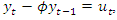 | (1) |
 is white noise with mean 0 and variance
  as
as | (2) |
 on the current value
  is only temporary and vanishes as
  if
if  In contrast, if
  we have
 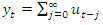 | (3) |
 on
on  is therefore persistent. In the former case,
  is a stationary autoregressive (AR) process of order 1 with variance
  | (4) |
 of size n, it is often extremely difficult to distinguish between the two cases. Indeed, there is hardly any difference between the two samples of size
  shown in Figure 1.a
  and Figure 1.c
  respectively. At first glance, both look nonstationary. The situation improves when the sample size is increased to
  . While the sample from the random walk still looks nonstationary (see Figure 1.b), the sample from the AR process now looks quite stationary (see Figure 1.d). In practice, the dataset is given and can usually not be increased arbitrarily. Only if we are lucky and the parameter
  of the data generating process is sufficiently smaller than 1 for the given sample size, the unit root hypothesis
  | (5) |
 | (6) |
 we can always choose a suitable value for the parameter
  so that the sample will look stationary even if
  (see Figure 1.h). This is due to the fact that the terms in the numerator and denominator of the lag polynomial representation
  | (7) |
 is chosen only slighty greater than -1. Thus, we can never be sure whether a rejection of the unit root hypothesis is due to a small value of
  or a value of
  close to -1 (for a more thorough line of reasoning see Pötscher, 2002).
 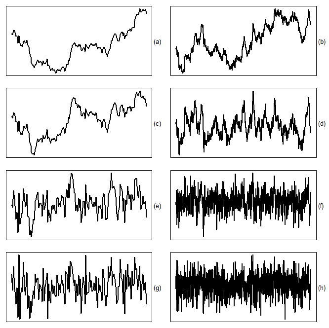 | Figure 1. Realizations of lengths 150 (first column) and 1000 (second column), respectively, of a random walk (first row), an AR(1) process with = 0.95 (second row), an AR(1) process with = 0.5 (third row), and an ARMA(1,1) process with = 1 and θ = -0.99 (fourth row) |
 | (8) |
 is negative in both cases (see Figures 2.b and 2.f), only the second cumulative plot shows a clear downward trend. However, this visual significance is somewhat put into perspective when higher-order lags are also considered (see Figures 2.c and 2.g). All computations are carried out with the free statistical software R (R Core Team, 2018).Unfortunately, overdifferencing can also occur in the case of a nonstationary time series. When we consider the general class of autoregressive fractionally integrated moving average (ARFIMA) processes
  | (9) |
 and I(0) processes, i.e., processes that are integrated of order zero
  but there are also processes that are fractionally integrated. For stationarity, it is required that
  Our goal is to distinguish stationary processes with
  which include white noise processes as well as AR, MA and ARMA processes, from nonstationary processes with
  which include random walks as well as ARIMA processes. We have seen above that a negative autocorrelation can be an indication of overdifferencing. Taking first differences reduces the memory parameter
  by 1. In the case of an I(1) process, the memory parameter decreases from one to zero and is therefore still nonnegative whereas in the case of an I(0) process, it decreases from 0 to -1. In contrast, both in the case of a fractionally integrated process with
  which is stationary, and in the case of a fractionally integrated process with
  which is nonstationary, the memory parameter will become negative after differencing. Checking for negativity after differencing is therefore pointless. An obvious alternative is fractional differencing with the help of the fractional differencing operator, which is defined as a power series expansion in integer powers of
  i.e.,
i.e., | (10) |
 in (10) will reduce the memory parameter by 0.5, hence we will observe overdifferencing exactly in the stationary case where the original order of integration is less than 0.5. Fractional differencing with
  can also help to detect underdifferencing. For example, when a strong positive autocorrelation is not only present in the original, not differenced series (see, e.g., Figures 2.d and 2.h) but also after fractional differencing, albeit to a lesser extent.
 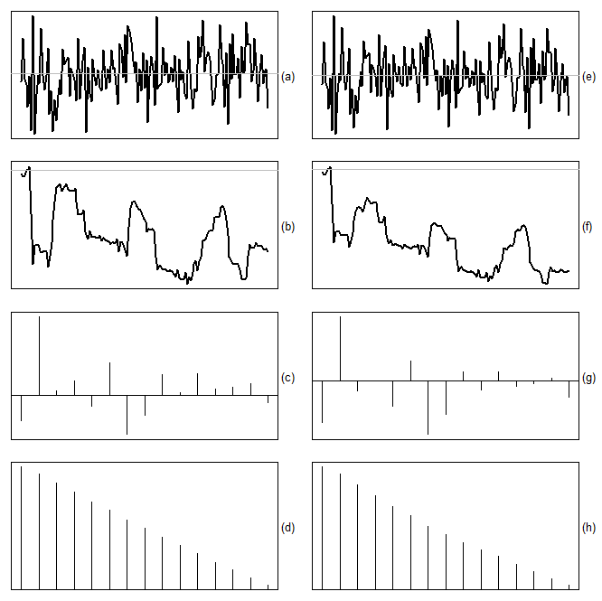 | Figure 2. Random walk (first column) vs. AR(1) process with = 0.95 (second column): (a), (e): First differences, (b), (f): First-order sample autocovariance plotted cumulatively, (c), (g) Sample autocovariances, (d), (h): Sample autocovariances of original series |
 by truncation, we will construct in Subsection 2.3 another approximation which is based on a parsimonious ARMA(1,1) model. But before that we will in the next subsection briefly leave the time domain and switch to the frequency domain where root differencing is a trivial exercise.
 2.2. Analysis in the Frequency-Domain
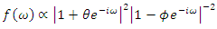
- The spectral density of an ARFIMA process is given by
 | (11) |
 either goes to infinity
  or to zero
 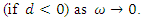 Only in the case of a pure ARMA process
  it converges (horizontally) to a positive number. After root differencing, the spectral density goes to zero if and only if
  i.e., exactly in the case of stationarity. In the frequency domain, root differencing can be accomplished simply by multiplying the spectral density by the factor
  | (12) |
 Nonparametric estimates of the spectral density can be obtained by smoothing the periodogram
 | (13) |
 A more elaborate method is the log periodogram regression which is based on the low-frequency approximation
  | (14) |
 we must replace the spectral density in this approximation by the periodogram (see Geweke and Porter-Hudak, 1983) or a smoothed version of it (see Hassler, 1993, Peiris and Court, 1993, and Reisen, 1994) and choose a suitable neighborhood
  of frequency zero. The parameter
  determines how many of the lowest Fourier frequencies are included in the regression (for a procedure involving non-Fourier frequencies, see Reschenhofer and Mangat, 2021). As always, there is a trade-off between bias and variance. A small value of
  increases the variance whereas a large value of
  may introduce a bias caused by short-term autocorrelation. In order to illustrate the frequency-domain approach outlined above, we consider a financial application where
  is known a priori. Although stock price series cannot adequately be modeled by a random walk (and not even by a conditionally heteroskedastic random walk with drift), there is a broad agreement that they are integrated of order 1, hence
  A disadvantage of financial datasets is that they are usually very short. Stock prices are rarely available for hundred years or more. A large sample size is not helping in this regard. E.g., for the investigation of climate change, a long annual temperature series from 1850 to 2020
  is certainly more appropriate than a short daily series from 2001 to 2020
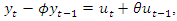
  Indeed, Figure 3 shows that simply increasing the resolution of a time series does not change the shape of the periodogram in the low-frequency range. For each frequency, annual (3.a), monthly (3.b), and daily (3.c), the scatter plot based on the low-frequency relationship approximation (14) corroborates our suspicion that
  Moreover, after multiplication by the factor (12), the periodograms still increase as
  (see 3.d-f), which is inconsistent with stationarity of the original series.
 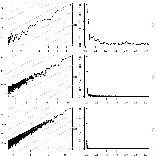 | Figure 3. For each frequency (first row: annual, second row: monthly, third row: daily), we first plot the log periodogram of the log S&P 500 from 1928 to 2020 against  and compare it to dashed lines of slope 1 and then we plot the root differenced periodogram against and compare it to dashed lines of slope 1 and then we plot the root differenced periodogram against  |
2.3. Approximating the Root Differencing Operator
- Usually, we interpret an ARMA equation such as (6), which can in lag operator notation also be written as
 | (15) |
 to a more complex process
  In the frequency domain, this transformation is accomplished by multiplying the constant spectral density
 | (16) |
 | (17) |
 | (18) |
 to a possibly stationary process
  The spectral density of
  is obtained from the spectral density of
  by multiplication with the factor
 | (19) |
 | (20) |
 | (21) |
 must be smaller than
  or else the decline will vanish completely. The result of the dampened differencing is then given by
 | (22) |
 | (23) |
 we need to find suitable values of
  and
and  so that a plot of the log of (23) against
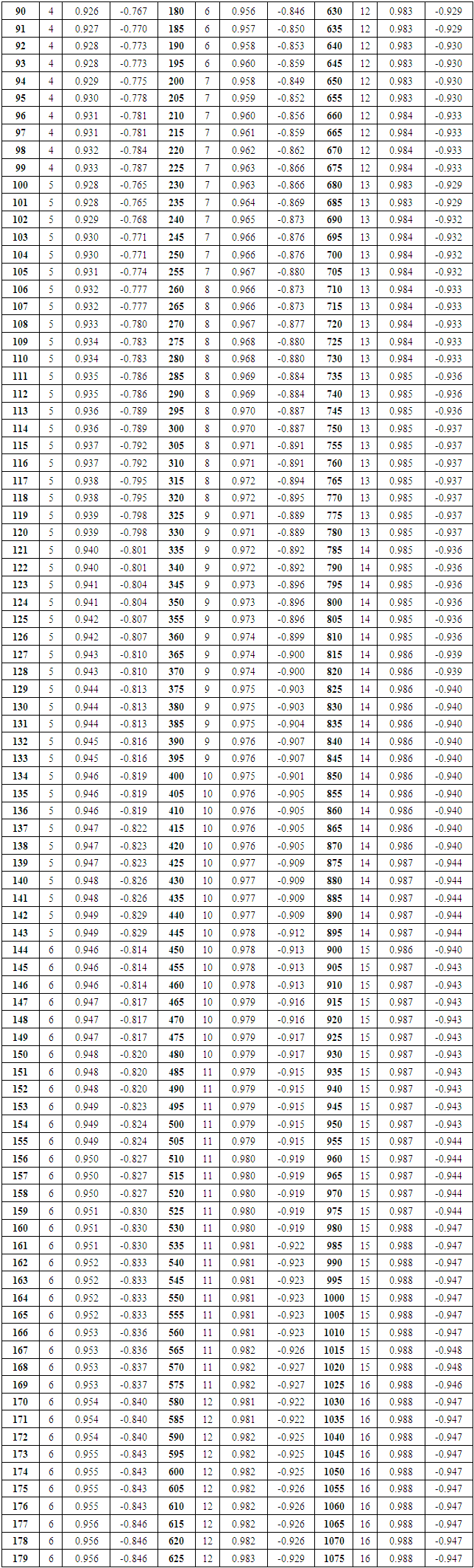
  has approximately a slope of 0.5 in the neighborhood of frequency zero. Table 1 gives pairs of values of
  and
and  for various sample sizes which mimic the effect of root differencing. These values were found by minimization of
 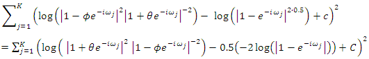 | (24) |
 and
and  where
where  The values in Table 1 can also be used for the approximation of the root integration operator
  which is just the inverse operator of the root differencing operator
  Indeed, if
  is obtained from
  by approximate root differencing, i.e.,
  | (25) |
 can be obtained from
  by approximate root integrating, i.e.,
  | (26) |
|
 (sample size, number of lowest Fourier Frequencies used for fitting,
 | (27) |
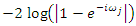 in Figures 4.b, e, h. Of special interest is the low frequency range (see Figures 4.a, d, g), where the graphs are approximately linear with slope 0.5. In this frequency range, the fit obtained by truncated series approximations is generally worse (see Figures 4.c, f, i). In the following, we will therefore change our setting slightly to make up for the shortcomings of the latter approximation. Firstly, we will introduce an initial settling period of length
  and thereby reduce the analysis period from
  Secondly, we will use an expanding cut-off lag instead of a fixed one.
  | Figure 4. For sample sizes  (first row), 250 (second row), and 1000 (third row), selected log ARMA(1,1) spectral densities are plotted against (first row), 250 (second row), and 1000 (third row), selected log ARMA(1,1) spectral densities are plotted against 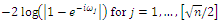 (first column) and (first column) and 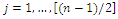 (second column), respectively, and are then compared to dashed base lines with slope 0.5. Note that the low frequencies appear on the right side! The spectral shapes in the third column were obtained by truncated series approximations of the root differencing operator with cut-off lags 20 (blue) and 50 (red), respectively (second column), respectively, and are then compared to dashed base lines with slope 0.5. Note that the low frequencies appear on the right side! The spectral shapes in the third column were obtained by truncated series approximations of the root differencing operator with cut-off lags 20 (blue) and 50 (red), respectively |
 and
and  respectively, are overdifferenced as indicated by a log periodogram that decreases as the frequency decreases (see Figures 5.8, 9, 17, 18), and that a root differenced fractional series with
  is underdifferenced as indicated by a log periodogram that still increases as the frequency decreases (see Figures 5.25, 26). These findings are also in line with the results obtained by root differencing in the frequency domain (see Figures 5.7, 16, 25). Moreover, there is also agreement that the strong positive autocorrelation, which is present in the fractional series with
  (see Figure 5.22), is (to a lesser extent) still present after root differencing (see Figures 5.23, 24). In contrast, the analogous plots for the stationary series are inconclusive (see Figures 5.4-6, 13-15). However, the truncated series approximation has at least managed to produce a negative first-order autocorrelation in each case (Figure 5.6, 15). In general, this method appears to remove a possible (stochastic) trend slightly more aggressively than the ARMA(1,1) approximation (see Figures 5.1-3, 20-12, 19-21).
 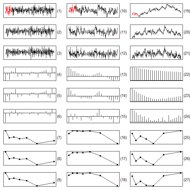 | Figure 5. Analysis of fractional series with  (3rd column): 1st row: Realizations with initial settling period (red, n=30) and analysis period (black, n=220); 2nd row: Root differenced series obtained with ARMA(1,1) approximation; 3rd row: Root differenced series obtained with truncated series (expanding cut-off lag); Rows 4-6: Sample autocorrelations of the original series and the two root differenced versions; Rows 7-9: Log periodogram plots (3rd column): 1st row: Realizations with initial settling period (red, n=30) and analysis period (black, n=220); 2nd row: Root differenced series obtained with ARMA(1,1) approximation; 3rd row: Root differenced series obtained with truncated series (expanding cut-off lag); Rows 4-6: Sample autocorrelations of the original series and the two root differenced versions; Rows 7-9: Log periodogram plots  for the root differenced series; (7: root differencing in the frequency domain, 8: ARMA(1,1), 9: truncated series) for the root differenced series; (7: root differencing in the frequency domain, 8: ARMA(1,1), 9: truncated series) |
3. Empirical Results
3.1. Global Warming
- There has been a broad and often controversial discussion about the true nature of the apparent upward trend in global surface temperature (see, e.g., Stern and Kaufmann, 1999; Fomby and Vogelsang, 2002; Kaufmann and Stern, 2002; Kaufmann et al., 2006; Kaufmann et al., 2010; Reschenhofer, 2013; Estrada et al., 2013; Estrada et al., 2017; Estrada and Perron, 2019; Lai and Yoon, 2018; Mangat and Reschenhofer, 2020; Chang et al., 2020). We add to this debate with an empirical study based on root differencing. Following the recommendation of the Climatic Research Unit (CRU) of the University of East Anglia (UEA), we use the HadCRUT5 dataset (Morice et al., 2021) for our investigation of the change of the global temperature since 1850. This dataset contains the global annual means from 1850 to 2020 of the combined land and marine temperature anomalies. Temperature anomalies are defined relative to the 1961–1990 temperature mean. The dataset is available at the website https://sites.uea.ac.uk/cru/data of the CRU. Although the observation period is not very long, we will again introduce an initial settling period of length
 The resulting reduction of the analysis period from 171 to 145 years can to some extent be justified by the fact that the global means of the first years are based on a significantly smaller number of measurements. In particular, this is true for the years before 1880. Note that a similar surface temperature dataset, namely the GISTEMP v4 (see GISTEMP Team, 2021; Lenssen, 2019) provided by the NASA (https://data.giss.nasa.gov/gistemp/), is only available from 1880.The central question is whether the recent rise in temperature is just a transient phenomenon or an indication of nonstationarity. Applying the methods used for the production of Figure 5 to our global surface temperature series, we find that all indications point to nonstationarity. Firstly, the root differenced series (obtained from the mean-corrected original series) still exhibit some kind of an upward trend (see Figures 6.d, g). Secondly, there is also strong positive autocorrelation left after root differencing (see Figures 6.e, h). Thirdly, the log periodogram of the root differenced series always increases as the frequency decreases, regardless whether root differencing is carried out in the frequency domain (see Figure 6.c) or in the time domain (see Figures 6.f, i).
 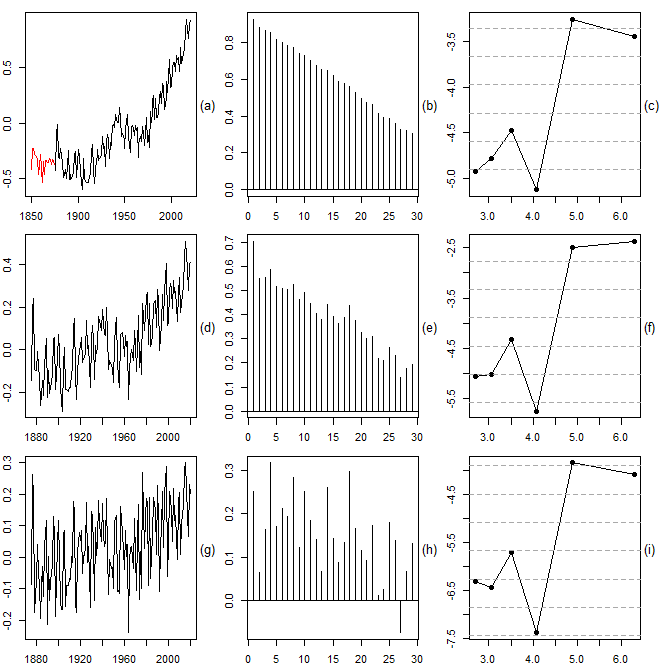 | Figure 6. Analysis of global surface temperature from 1850 to 2020 (HadCRUT5): 1st column: Plots of original (a) and two root differenced series (d: ARMA, g: truncated); 2nd column: Sample autocorrelations of original and root differenced series; 3rd column: Log periodogram plots after root differencing (c: frequency domain differencing) |
3.2. Economic Growth
- We downloaded the real UK GDP per capita since 1252 (in 2011$) from the Maddison Project Database (see Bolt and van Zanden, 2020; Scheidel and Friesen, 2009; Stohr, 2016), which is maintained by the Groningen Growth and Development Centre at the University of Groningen. The 2020 version of this database covers the period up to 2018. In contrast to the previous section, we take the logarithm of the data before we carry out the analysis. Again, the empirical results are in favor of nonstationarity, only much stronger. There is stunning evidence of underdifferencing (see Figure 7). Of course, this does not come as a surprise. In the case of economic growth, it is a priori clear that there is an upward trend. The only question is whether this trend is deterministic or stochastic. In the latter case, it is safe to assume that
 hence root differencing is definitely not enough.
 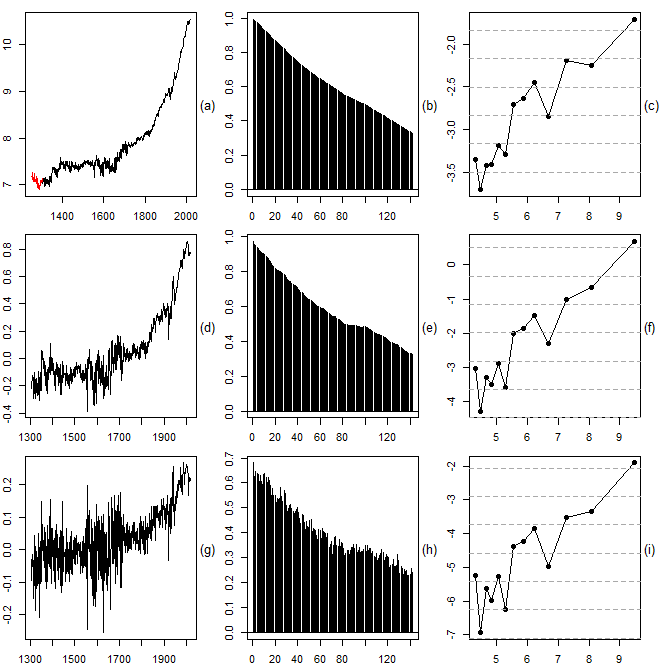 | Figure 7. Analysis of log UK GDP per capita from 1252 to 2018 (Maddison Project Database): 1st column: Plots of original (a) and two root differenced series (d: ARMA, g: truncated); 2nd column: Sample autocorrelations of original and root differenced series; 3rd column: Log periodogram plots after root differencing (c: frequency domain differencing) |
3.3. Migration
- We obtained Swedish migration data from 1851 until 1969 from Mitchell (2003) and from 1970 until 2020 from the website of Statistics Sweden (https://www.scb.se/). The main reasons for selecting Sweden in our analysis of migration dynamics included the existing availability of long historical time series as well as the recent upsurge in academic interest in the subject of migration and flight by Swedish scholars and organizations (Lindfors and Alfonsdotter, 2016, see also Warnqvist, 2018). Furthermore, compared to other European countries, Sweden is known to have had generous asylum laws until 2016. Much earlier already, Sweden became an immigrant country in the 1930s, after initial mass migratory movements toward the United States. This mass migration unfolded throughout different waves between the 1840s and the late 1920s. Applying the same methods as in the previous subsections, we again find evidence of nonstationarity, albeit somewhat weaker than before. The empirical findings are shown in Figure 8 for the immigration data and in Figure 9 for the emigration data. In both cases, it is safe to assume that the observed nonstationarity is mainly due to structural breaks which separate different waves of migration.
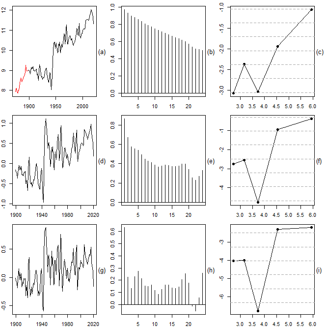 | Figure 8. Analysis of log Swedish immigration numbers from 1875 to 2020: 1st column: Plots of original (a) and two root differenced series (d: ARMA, g: truncated); 2nd column: Sample autocorrelations of original and root differenced series; 3rd column: Log periodogram plots after root differencing (c: frequency domain differencing) |
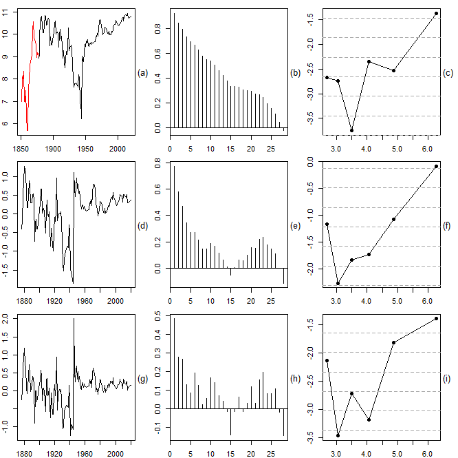 | Figure 9. Analysis of log Swedish emigration numbers from 1851 to 2020: 1st column: Plots of original (a) and two root differenced series (d: ARMA, g: truncated); 2nd column: Sample autocorrelations of original and root differenced series; 3rd column: Log periodogram plots after root differencing (c: frequency domain differencing) |
4. Discussion
- Carrying out fractional differencing with the help of a truncated version of the power series expansion of the fractional differencing operator is only meaningful when the sample size is very large. For more realistic sample sizes occurring in practice, we therefore propose a simple approximation which is based on a simple ARMA(1,1) model. We focus on the important special case where the fractional differencing parameter is equal to 0.5 (root differencing). This choice allows the use of the new method to distinguish between stationarity and nonstationarity of a given time series. For this purpose, we look at the time series plot, the sample autocorrelations, and the periodogram of the root differenced time series. A trend or long cycles in the plot, positive and slowly decaying sample autocorrelations, and a peak of the periodogram at frequency zero are interpreted as indications of nonstationarity. The new method is applied to long annual time series, the global surface temperature from 1850 to 2020 (HadCRUT5), the UK GDP per capita from 1252 to 2018 (Maddison Project Database), Swedish immigration numbers from 1875 to 2020 and Swedish emigration numbers from 1851 to 2020 (Mitchell, 2003; Statistics Sweden). In each case, we expect a priori that the hypothesis of stationarity is rejected. The temperature series and the GDP series have an upward trend because of global warming and long-term economic growth, respectively. The nonstationarity of the migration series is due to structural breaks which separate different waves of migration. It is reassuring that our empirical analysis of these series indeed produces evidence in favor of nonstationarity. However, this evidence is not always as strong as anticipated, which is particularly sobering in view of the fact that most historical time series are much shorter than the examples investigated in this paper. For example, studies of the long-term properties of macroeconomic time are usually based only on post-war data (see, e.g., Christiano and Eichenbaum, 1990; Hauser et al., 1999). Not helping in this matter would be to increase the frequency from annual to quarterly or monthly, which increases only the number of observations but not the length of the observation period. We conclude that even after refraining from carrying out a formal statistical test (because of inherent theoretical issues; see Pötscher, 2002) and turning to a more informal approach as described in this paper, it may still be hard to find reliable evidence in favor or against stationarity unless the observation period is extremely long.