1. Introduction

Recent reports from the World Health Organization (WHO) indicate that road traffic injuries (RTIs) account for about 1.3 million deaths worldwide annually [1,2]. Of particular concern is a continual increase of RTI rate of mortality [3]. Conclusions from recent investigations indicate that most RTI deaths occur prior to hospital arrival, either at the at the crash scene, or during patient transport [4,5], that 86 percent of trauma-related deaths occur in the pre-hospital phase [6], and that 39 percent of associated deaths are preventable [4,6]. Within the United States, motor vehicle crashes (MVC) also continue to be a leading cause of death and injury, in spite of important improvements to road infrastructure, vehicle design, and traffic safety legislation [7]. Because emergency medical services provide the critical link between injury and definitive critical care [8], the time between the occurrence of a MVC and delivery of a patient to this care is a vital factor in regard to the potential and probability of MVC mortality [9]. The importance of EMS travel delays and arrival times, and the strong connections between MVC’s, EMS Response Time (ERT), and patent mortality, are further illustrated by numerous additional studies [10-17].

EMS Response Time (ERT) is the travel time interval between the initial reporting of a crash and the arrival of EMS personnel at the crash site [18,19,20]. Many factors influence the magnitude of ERT, such as crash site location (rural, suburban, or urban), road conditions, weather conditions, locations of ambulances within the service zone, transportation times, measures of rurality, on-scene and transport times, access to trauma resources, and traffic safety laws [11,12,21,22]. Results for rural/wilderness locations, as well as for urban/suburban settings, indicate that 9.9% and 14.1% of crash fatalities, respectively, are associated with prolonged response times [12]. According to Byrne et al. [12], such mortality rates have important implications for trauma system design and health policy [12].

Related results are also provided by Eftekhari et al. [23] which show that poor management of time is one of the six major challenges related to preventable deaths in RTIs. According to Ma, et al. [24], ERT, in addition to age, gender, seating position, and manner of collision, are all statistically significant in regard to the possibility of a fatality. These researchers further indicate that “the marginal smooth influential pattern of the ERT is non-monotonic” in regard to the relationship between longer ERT and the probability of a death. He et al. [25] employ spatial regression methods to demonstrate that establishing EMS performance measures is critical for the improvement of a rural community's access to Emergency Medical Services. According to these investigators, low service coverage measure means that improved strategic establishment or relocation of service stations are needed.

The present investigation employs Geographically Weighted Regression (GWR) with two different kernel weighting functions: adaptive bi-square kernel and adaptive Gaussian kernel. Results from these functions are compared, for a wide range of experimental conditions, using ANOVA tables and analytic tools to determine the arrangement which gives the most physically realistic results. To provide a baseline reference comparison, resulting data are also considered relative to Global Regression Analysis (GRA) calculations. Crash records data for Pickens County Alabama for dates between January 2016 and December 2019 are used for this study. The impacts of the combination of six independent variables on the EMS Response Time (ERT) are modeled, including travel time, time of the day, day of the week, weather, lighting conditions, and crash severity. The present study is unique and different from previous studies because different kernel weighting functions are considered and employed with GWR, and because the present data are collected from a rural county in Alabama with only one EMS dispatch center.

2. Analytic Analysis Methods

2.1. Test Environment Data

Crash records for Pickens County Alabama are obtained from the Critical Analysis Reporting Environment (CARE) database. Pickens County is a county located on the west central border of the U.S. state of Alabama. The medical center for the Pickens County is located at 241, Robert K Wilson Dr., Carrollton, AL 35447. There is only one Emergency Medical Services (EMS) dispatch location within the entire county. The longitude and latitude coordinates for the EMS dispatch center are used as the hospital location. For the dates between January 2016 and December 2019, the total number of crashes reported is 214.

From the crash data, EMS response time (ERT), travel time, crash severity, day of the week, time of the day, lighting condition, and weather are considered as the variables for this study. Travel time is calculated between the Pickens County hospital location and each of the crash sites using Google Maps with travel time recorded in minutes for the fastest route. GWR4 software [26] is used to analyze the data using Global Regression Analysis (GRA), Geographically Weighted Regression (GWR) with an adaptive bi-square kernel weighting function, and Geographically Weighted Regression (GWR) with an adaptive Gaussian kernel weighting function. Figure 1 shows a map of Pickens County, with the hospital (EMS) location, and including four crash site locations.

Figure 1. Pickens County map with hospital (EMS) location and four examples of crash sites

2.2. Regression Analysis Using Geographically Weighted Regression (GWR)

Employed within the present investigation is GWR4 statistical software, which is specially developed for Geographically Weighted Regression (GWR) modeling [26]. Within this analytic code, a semi-parametric Gaussian GWR model is described using the equation given by

(1)

where y_i, x_k,i and ε_i are the dependent variable, kth independent variable, and the Gaussian error at the location i, respectively. Quantities (u_i,v_i) are the latitude and longitude coordinates of the ith location, and coefficients β_k (u_i ,v_i) are varying with location. As such, x_k,i are local variables. z_l,i is the ith independent variable with a fixed coefficient γ_l. Variables z_l,i do not vary with location, and are thus, global variables. With this configuration, the analytic model uses both geographically local terms and geographically global terms. For GWR analysis, β coefficients, for the local variables, are not constant like global variables. Each coefficient β value varies based on the geographical location. Hence, instead of a singular estimate for the coefficient, for the GWR results, the mean, standard deviation, minimum, and maximum values of each β coefficient are provided for the local variables. In contrast, for global variables, the coefficient estimate, standard error (SE) and the t-statistic values are provided. The standard error (SE) is an estimate of the standard deviation of the coefficient for all considered test cases. Standard error is thus a measure of the precision with which the regression coefficient is measured. The t-statistic is the coefficient estimate divided by the associated standard error. As such, the t-statistic value indicates how strongly each independent variable is associated with the dependent variable, as given by

(2)

where t_k, β_k, and SE_k are the t-statistic, coefficient estimate, and standard error of the kth independent variable.

2.3. Weighting Functions for Geographically Weighted Regression (GWR)

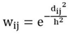
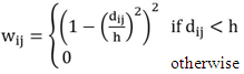
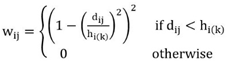
In GWR modeling, local parameters for each location are estimated based upon observations from nearby locations. Parameters associated with a location are more strongly affected by the observations occurring close by, relative to observations which are farther away.

The influence factor to account for such variations in regard to location is the weighting function, w_ij. Observations are considered to be crash data for one particular location. The weighting function value for each crash data case indicates the influence of this case on the regression estimate of a different crash case. The weighting function value of cases closer to a particular crash location is then higher than the weighting function value of cases which are farther away.

Two commonly used kernel weighting functions for this purpose are Gaussian and bi-square, as expressed using the following equations.

Fixed Gaussian:

(3)

Fixed bi-square:

(4)

Adaptive bi-square:

(5)

Adaptive Gaussian:

(6)

Within Eqns. (3)-(6), i is the regression point index, j is the locational index, w_ij is the weight value of observation at location j for estimating the coefficient at location i, and d_ij is the Euclidean distance between i and j. Parameter h is a fixed bandwidth size, defined by a distance metric measure, and h_i(k) is an adaptive bandwidth size defined as the kth nearest neighbor distance.

Both Gaussian and bi-square kernel functions incorporate a distance decay function which allocates more weight to properties closer to a regression point compared properties located farther away. If a fixed kernel function is selected, the geographic extent for local model fitting to estimate geographically local coefficients is constant over space. On the other hand, adaptive kernel functions change locally by controlling the kth nearest neighbor distance for each regression location.

With GWR, the size of the bandwidth is optimized by either distance (fixed kernel) or the number of neighboring observations (adaptive kernel). Gaussian kernel weight continuously and gradually decreases from the center of the kernel but never reaches zero. Such a Gaussian kernel is suitable for fixed kernels since it can mitigate the possibility of no data within a kernel range of values. A bi-square kernel function then has a defined range, where kernel weighting is non-zero, and is thus useful to clarify local extents for model fitting.

2.4. Regression Analysis Approach - Global Regression Analysis (GRA)

In contrast to GWR, Global Regression Analysis or GRA does not account for geographical variability. For this approach, the model is given by the following equation

(7)

where y_i, x_k,i and ε_i are dependent variable, kth independent variable, and the Gaussian error, respectively. Hence, the value of the estimate is the coefficient β for the corresponding variable.

The regression intercept value is the mean for the dependent variable when all independent variables are equal to 0. The intercept is needed to determine predicted values. For GWR results, the intercept term is generally specified as a local varying term since other coefficients often cause a variation of the intercept. Note that a regression without an intercept value indicates that the regression line goes through the origin, wherein the dependent variable and the independent variable are both equal to zero.

3. Analytic Results

3.1. Results Using Geographically Weighted Regression (GWR) with Adaptive Gaussian Kernel Weighting Function

Here, results are obtained using GWR with an adaptive Gaussian kernel weighing function, as expressed using Eqn. (6). With this arrangement, Gaussian kernel weight continuously and gradually decreases from the center of the kernel, but never reaches zero. Longitude and latitude of the crash site are used for location data. ERT is the dependent variable. Independent variables are day of the week, time of the day, weather, crash severity, lighting conditions, and travel time. Based on the geographical variability results, all the independent variables except travel time are local terms.

Variance inflation factor (VIF) values are also determined for different combination of variables. The VIF value quantifies the severity of multi-collinearity within least squares regression analysis results. The present VIF values are calculated using R-Square values obtained using Analysis ToolPak within Microsoft Excel software. Resulting VIF values for multiple combinations of variables from the present study range between 1.0002 and 2.0943. Because these VIF values are close to one and very low compared to 5, the six independent variables are not strongly correlated with each other. Note that VIF values greater than 5 indicate that multi-collinearity between parameters (or variables) is high.

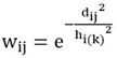
3.1.1. Travel Time - Global Independent Variable

Table 1 shows GWR results for ERT as the dependent variable and travel time as only one independent variable. The effect of travel time on ERT is indicated by the coefficient estimate, which is positive indicating that ERT increases with an increase in the travel time. According to the coefficient value, the average ERT is 1.1% longer than actual travel time when no other independent variables are considered. The standard error (SE), which indicates the variation of estimate, is 0.257. The t-statistic value is for travel time is 3.939. This magnitude of t-statistic indicates that travel time has a significant impact on the EMS response time (ERT). The value of the intercept is not significant for the analysis, because variables are quantified using code numbers.

Table 1. Results obtained using Geographically Weighted Regression (GWR) with an adaptive Gaussian kernel weighing function for EMS response time (ERT) as dependent variable and travel time as only one independent variable

3.1.2. Travel Time - Global Independent Variable with Other Local Independent Variables

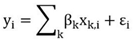
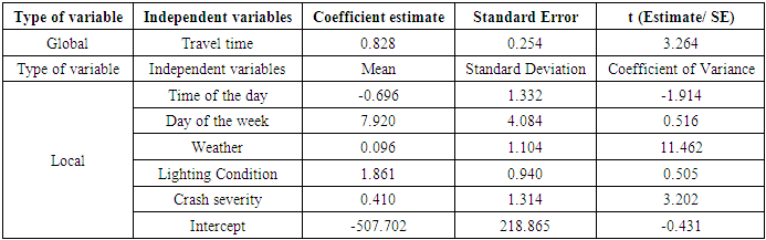
Tables 2a-2c show GWR results for ERT as the dependent variable and travel time as one independent variable, with additional independent variables added to the analysis. According to these data, travel time always has a positive impact on the ERT, such that, as travel time increases, the ERT also increases. The coefficient of the variable travel time ranges between 0.828 and 1.020, as different independent variables are added to the analysis. The coefficients also indicate that ERT is shorter than travel time for most of the combinations of variables. Data from Tables 2a-2d also show that the impact of travel time on ERT variation is very small, as other variables are added to the analysis. Adding variables time of the day, lighting conditions, weather, and crash severity to the analysis reduces the coefficient estimate for travel time. In contrast, adding variable day of the week increases the coefficient estimate value.

Table 2a. Results obtained using Geographically Weighted Regression (GWR) with an adaptive Gaussian kernel weighing function for EMS response time (ERT) as dependent variable and travel time as one independent variable with two additional independent variables

Table 2b. Results obtained using Geographically Weighted Regression (GWR) with an adaptive Gaussian kernel weighing function for EMS response time (ERT) as dependent variable and travel time as one independent variable with three additional independent variables

Table 2c. Results obtained using Geographically Weighted Regression (GWR) with an adaptive Gaussian kernel weighing function for EMS response time (ERT) as dependent variable and travel time as one independent variable with five additional independent variables

The t-statistic value greater than 1 indicates that the coefficient estimate is larger than the standard error, which indicates that the independent variable has a significant influence on the dependent variable. The t-statistic value for variable travel time ranges between 3.264 and 4.064. This indicates that travel time has a significant impact on the EMS response time (ERT) value. The t-statistic magnitude for travel time increases by adding variable day of the week to the analysis. In contrast, including variables time of the day, lighting condition, weather, and crash severity to the analysis slightly reduces the t-statistic value.

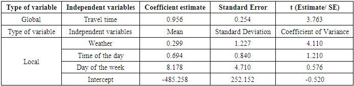
3.2. Global Regression Analysis (GRA) Results

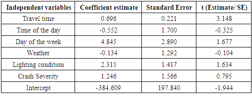
Global Regression Analysis (GRA) does not account for variations due to spatial location, which means that associated model results are generally independent of location. Estimated coefficient values are thus spatially-averaged global values, and all independent variables are global. Within the present investigation, results obtained with this approach (without location influences) are used for comparison.

Table 3 shows results for ERT as dependent variable with one independent variable. Table 4 shows results for ERT as dependent variable and travel time as one independent variable with five additional independent variables. For both sets of data, the coefficient of travel time is always lower than one. Results in Table 4 indicate that travel time, time of the day, and day of the week have a positive impact on ERT, which is qualitatively similar to GWR analysis results. Evidence is also provided by Table 4 data that weather has a negative impact on ERT.

The t-estimate values for travel time, from Tables 3 and 4, are 3.425 and 3.148, respectively. In Table 4, t-statistic values for lighting condition and day of the week show that these two variables have a significant impact on ERT. Weather and time of the day have a lower t-statistic value which indicates minor impact on ERT. As mentioned, the magnitude of the t-statistic value indicates the importance of the independent variable, such that a value greater than 1 indicates that the independent variable has a significant impact on the dependent variable.

Table 3. Results obtained using Global Regression Analysis (GRA) for EMS response time (ERT) as dependent variable with one independent variable

Table 4. Results obtained using Global Regression Analysis (GRA) for EMS response time (ERT) as dependent variable and travel time as one independent variable with five additional independent variables

Based on the coefficient estimates, when six independent variables are considered, data indicates that travel time has a greater influence on ERT with GWR analysis than with the GRA approach. Lighting condition, and crash severity have higher influence with GRA than the GWR model. The t-statistic values in Table 4 show that variables travel time, crash severity, lighting condition, and day of the week have statistically significant impacts upon ERT, whereas variables weather, and time of day have lower significance.

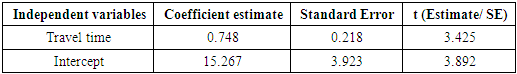
3.3. Comparisons of GRA Results, GWR Results with an Adaptive Gaussian Kernel Weighting Function, and GWR Results with an Adaptive Bi-Square Kernel Weighting Function

Figures 2-7 show variations of the coefficient for each independent variable, as additional variables are added, for GRA, and GWR analyses with both kernel weighting functions. Note that the value of the coefficient is averaged, as different variable combinations are employed, when two and three variables are considered.

Figure 2 shows that the coefficient for travel time varies only slightly as additional variables are added, for up to 3 variables. Somewhat larger variations are evident as the number of variables exceeds 3, for all three analysis approaches. For each variable number, GRA gives the lowest coefficients, whereas GWR with an adaptive bi-square kernel weighting function gives the highest coefficients. For all three analysis methods, Figure 3 shows that the coefficient for time of the day decreases in a progressive fashion, as additional variables are considered. Here, GRA coefficient values are consistently higher for all variable numbers, when compared to both GWR analysis methods. All three analysis methods give positive coefficients when up to four variables are employed, and negative values when a total of 6 variables are utilized.

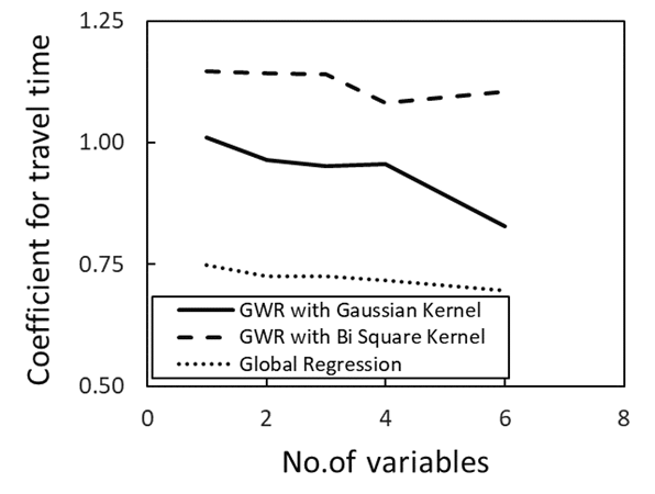Figure 2. Coefficient for travel time variation as additional variables are added, determined using GRA, GWR with Adaptive Gaussian Kernel Weight Function, and GWR with and Adaptive Bi-Square Kernel Weighting Function

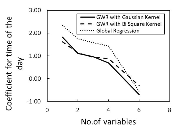Figure 3. Coefficient for time of the day variation as additional variables are added, determined using GRA, GWR with an Adaptive Gaussian Kernel Weighting Function, and GWR with an Adaptive Bi-Square Kernel Weighting Function

Figure 4 shows the variation of coefficient for day of the week as additional variables are added for all three analysis methods. Coefficient values are consistently positive for all three methods and for all variable numbers, such that the highest values are associated with GWR with an adaptive Gaussian kernel weighting function, and the lowest values are associated with GRA. The variation of coefficient for weather is shown in Figure 5 as additional variables are added. Here, coefficients are mostly positive for both GWR analysis approaches, but mostly negative when GRA is utilized. The highest values, as additional variables are added, are associated with GWR with an adaptive Gaussian kernel weighting function. Figures 6 and 7 show variations of coefficients for lighting conditions and crash severity, respectively, as additional variables are added. Associated coefficients are consistently positive for all analysis methods and variable numbers, where the highest value for each variable number is associated with the GRA analysis method.

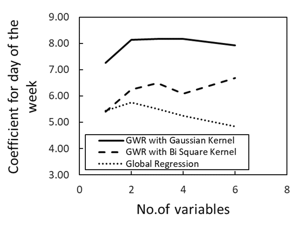Figure 4. Coefficient for day of the week variation as additional variables are added, determined using GRA, GWR with an Adaptive Gaussian Kernel Weighting Function, and GWR with an Adaptive Bi-Square Kernel Weighting Function

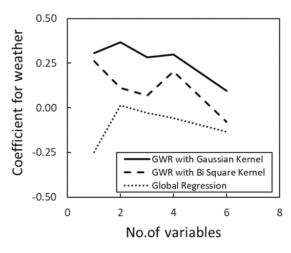Figure 5. Coefficient for weather variation as additional variables are added, determined using GRA, GWR with an Adaptive Gaussian Kernel Weighting Function, and GWR with an Adaptive Bi-Square Kernel Weighting Function

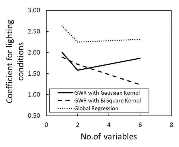Figure 6. Coefficient for lighting conditions variation as additional variables are added, determined using GRA, GWR with an Adaptive Gaussian Kernel Weighting Function, and GWR with an Adaptive Bi-Square Kernel Weighting Function

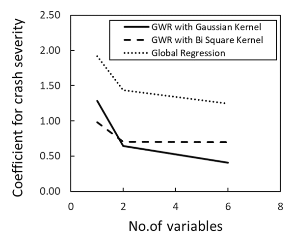Figure 7. Coefficient for crash severity variation as additional variables are added, determined using GRA, GWR with an Adaptive Gaussian Kernel Weighting Function, and GWR with an Adaptive Bi-Square Kernel Weighting Function

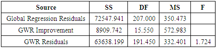
3.4. ANOVA Comparisons of GRA Results, GWR Results with an Adaptive Gaussian Kernel Weighting Function, and GWR Results with an Adaptive Bi-Square Kernel Weighting Function

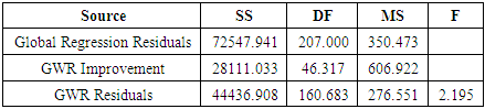
ANOVA, or analysis of variance, results are provided to compare the performance characteristics of GRA, GWR with an Adaptive Gaussian Kernel Weighting Function, and GWR with an Adaptive Bi-Square Kernel Weighting Function. As results from these different analysis methods are compared, ANOVA values indicate if adding geographical variability location data leads to significant improvements in model performance. With the ANOVA approach, determined are Source, Sum of Squares (SS), Degrees of Freedom (DF), Mean Square (MS), and F-statistic values. Values of SS are calculated for GRA and GWR residuals, and the difference between the GRA residual and the GWR residual is the GWR improvement. The MS value of GWR improvement, divided by the MS value of the GWR residual, is then the F-statistic.

Table 5 shows the ANOVA Table for geographically weighted regression (GWR) analysis with bi-square kernel weighting function, with six independent variables. The table indicates that SS is lower for GWR than for GRA, with a GWR improvement of 28111. Such characteristics mean that the GWR model provides a better fit to data, with more physically representative results. The MS value of the GRA model is 350.473. The MS value of the GWR model with a bi-square kernel function is 276.551. The F-statistic within Table 5 is 2.195. Because the MS value is lower, improved performance of the GWR model (with a bi-square function) is again indicated, relative to the GRA model.

Table 5. ANOVA Table for geographically weighted regression (GWR) analysis with bi-square kernel weighting function, with six independent variables

Table 6 shows the ANOVA Table for geographically weighted regression (GWR) analysis with Gaussian kernel weighting function, with six independent variables. The table shows that SS is lower for GWR than for GRA, with a GWR improvement of 8909. The MS value of the GWR model with a Gaussian kernel function is 332.401. The F-statistic within Table 6 is also greater than one, with a value of 1.724. Both characteristics indicate improved performance for the GWR model (with a Gaussian function), relative to the GRA model.

Table 6. ANOVA Table for geographically weighted regression (GWR) analysis with Gaussian kernel weighting function, with six independent variables

Comparing values in Tables 5 and 6 indicates that better modelling is provided using the bi-square kernel weighting function, compared to using the Gaussian kernel weighting function, since the associated MS value is lower. Note that results in Tables 5 and 6 both evidence improved model performance with the inclusion of geographical variability location data.

Note that Yacim, and Boshoff [27] also compare and discuss kernel function selection in geographically weighted regression.

4. Summary and Conclusions

EMS response time (ERT) variation for data for a rural county in west Alabama, Pickens County, is investigated for a total of 214 crash cases for the dates between January 2016 and December 2019. The choice of this test environment is unique because only one EMS dispatch center is located within the county. The present investigation is undertaken to demonstrate and compare the use of Geographically Weighted Regression (GWR) using two different kernel weighting functions: adaptive bi-square kernel and adaptive Gaussian kernel. These two weighting functions are considered to provide different analytic tools to account for geographical variability location data. To provide a baseline reference comparison, resulting data are also considered relative to Global Regression Analysis (GRA) calculations, which are obtained without the inclusion of geographical variability location analysis. Considered are different combinations of six independent variables. Based upon geographical variability results, day of the week, time of the day, weather, crash severity, and lighting conditions are local independent variables, and travel time is a global independent variable.

Results from GWR analyses, using both weighting functions, show important quantitative and qualitative differences in regard to coefficient values as each independent variable is individually addressed, especially as the number of considered variables is altered, relative to the addressed variable. From GWR ANOVA table data, values of SS are lower for GWR, using both kernel weighting functions, compared to GRA, with substantial GWR improvement values. Such characteristics mean that both GWR models provide a better fit to data, with more physically representative results. ANOVA table F-statistic and MS value data indicate that GWR analysis, with an adaptive bi-square weighting function, often yields improved model performance, relative to GWR with an adaptive Gaussian kernel weighting function. ANOVA table F-statistic data also evidence improved model performance, with the inclusion of geographical variability location data. This conclusion is based upon the result that both GWR analysis tools provide a lower MS value, indicating better performance relative to the GRA tool.

With the adaptive Gaussian kernel weighting function, all observations are considered, with weightings that tend towards zero as distance from the travel location increases. The adaptive bi-square approach gives observations with decreasing weight with distance, such that weight is zero beyond a certain distance h, called the bandwidth. Based on standard deviation data, the adaptive Gaussian kernel weighting function provides adequate representation of physical behavior for some experimental conditions. However, function values for observations beyond a certain distance are often inaccurate, resulting in unrepresentative coefficient values. Because of these issues, GWR with an adaptive bi-square kernel weighting function provides data which are physically more accurate for a wider range of experimental conditions.

Overall, the GWR and GRA analysis results indicate that, as the travel time increases, the EMS response time also increases. When different local independent variables are considered, EMS response time is larger on weekends than on weekdays. The EMS response time is larger in the evening and at night, when compared to morning. When the weather is clear or cloudy, the EMS response time is shorter. But when the weather is extreme, with mist, fog, or rain, the EMS response time is longer. When roads are dark, the EMS response time is longer, and when daylight is present, the EMS response time is shorter. If the crash is fatal, the EMS response time is longer compared to situations when crash injuries are non-severe.