-
Paper Information
- Next Paper
- Paper Submission
-
Journal Information
- About This Journal
- Editorial Board
- Current Issue
- Archive
- Author Guidelines
- Contact Us
International Journal of Statistics and Applications
p-ISSN: 2168-5193 e-ISSN: 2168-5215
2021; 11(3): 61-69
doi:10.5923/j.statistics.20211103.02
Received: Aug. 11, 2021; Accepted: Aug. 30, 2021; Published: Sep. 26, 2021

Identifying and Classifying Traveler Archetypes from Google Travel Reviews
 Abstract
 Reference
 Full-Text PDF
 Full-text HTML
Mst Sharmin Akter Sumy1, 2, Md Yasin Ali Parh1, 2, Md Sazzad Hossain2
1Department of Bioinformatics and Biostatistics, University of Louisville, Louisville, KY
2Department of Statistics, Islamic University, Kushtia, Bangladesh
Copyright © 2021 The Author(s). Published by Scientific & Academic Publishing.
This work is licensed under the Creative Commons Attribution International License (CC BY).
http://creativecommons.org/licenses/by/4.0/

We investigated how grouping consumers with similar interests is important for revenue optimization. A real dataset application is carried out to see this importance. To identify traveler archetypes from Google travel reviews Principal components analysis, hierarchical clustering, and k-means clustering were used in this article. K-nearest neighbors were used to classify the identified classes in the dataset. The results confirmed that, these prediction algorithms have high accuracy measures, but the clustering methodologies require further improvement. The classes identified should be checked by a domain expert for reasonableness before practical application. Because of the unlabeled data, it was not possible to test the model on new data. This model could be deployed on a small subset of customers and data could be collected on the performance of business metrics.
Keywords: Google review, Revenue optimization, Clustering methodologies
Cite this paper: Mst Sharmin Akter Sumy, Md Yasin Ali Parh, Md Sazzad Hossain, Identifying and Classifying Traveler Archetypes from Google Travel Reviews, International Journal of Statistics and Applications, Vol. 11 No. 3, 2021, pp. 61-69. doi: 10.5923/j.statistics.20211103.02.
Article Outline
1. Introduction
- The way that customers find and choose businesses has changed drastically in recent years. In the past, consumers would rely mainly on a business’s advertising, previous experience, or recommendations from family and friends. Now a days, more and more people turning to local search Google and starting to automatically filter out local businesses. People are able to go online and list their thoughts about the company without having to download an app.Google reviews allow technology firms to prove themselves to their potential customers. Big or small, the business who takes advantage of Google reviews is in a position to rank higher in local search results. The reviews level the playing field where advertising, expensive campaigns less relevant. Of course, those same campaigns and advertising can certainly have a huge impact. But they become less relevant in the context of Google business reviews, since reviews serve as transparency and social proof rather than beautiful marketing. With proper execution, Google reviews can be one of the most successful marketing tactics. This is partially because Google reviews allow technology firms to show up in the “Map Pack.” With an increase of 19.9% in 2016 and a forecasted growth of 17.5% for 2017, global business to consumer (B2C) e-commerce is now accounting for 8.7% of retail sales worldwide. [1] The effect of consumer reviews on online decisions is widely recognized. Numerous studies have shown that consumer ratings and reviews impact people's purchasing behavior and intentions, as well as attitudes towards products and retailers. [2] [3] [4]Although positive and negative reviews can sway consumers' behavior, some research has indicated that they differ in their impact. Negative reviews can significantly influence subsequent opinion in a positive way if those responses are observable at the time of reviewing. [5] Purnawirawan et al. [6] reported that negative reviews had the strongest effect on attitudes and usefulness, suggesting that negative reviews may carry more weight than positive reviews [7], [8]. Online platforms often provide consumer reviews in two formats: average ratings and single review. Average rating giving an overview over the overall perceived quality (i.e., statistical information) and single reviews that contain personal narratives of experiences made with a specific product. A recent consumer survey indicated that customers rate average ratings as most important [9] Hong and Park [10] found that both statistical information and narrative information are equally convincing. It is important to see how average user rating helps technology farms to reduce advertising cost. Identification of consumer subcategories is a very powerful tool for optimizing advertising revenue at large technology firms. Thus, the main objective of this article was to identify and classify Google users into traveler archetypes. Data used for this task were average Google reviews of various travel locations and amenities. Archetypes were then predicted using a variety of statistical learning methods based on the existing data. The paper can be divided into three main parts. A discussion of the unsupervised statistical learning techniques used to identify traveler archetypes is presented first. The methods used to predict these archetypes are presented second. Finally, findings and further considerations for the work are detailed.
2. Methods
- There were three main phases of the analysis. First, an exploratory analysis was conducted to understand the dataset and detect any relationships that may prove useful later. Second, unsupervised learning methods were used to understand the structure of the data and assign traveler archetypes. This phase of the research is the most critical to its success as the results of this analysis were used in later methods. Finally, supervised learning methods were built on the constructed class structures. The specific learning methods employed in each portion of the article are presented below.
2.1. Data
- The dataset consists of average Google review from 5454 distinct individuals across 24 distinct travel amenities and leisure businesses. Each review is on an ascending scale of 0 to 5. Table 1 in the appendix contains a complete description of variables contained in the dataset. This data was obtained from the University of California, Irvine’s Machine Learning Dataset Repository. [11]
2.1.1. Exploratory Analysis
- An important question during the exploratory analysis was whether the data should be centered and scaled for use in unsupervised learning methods. Examination of univariate plots of the average reviews proved useful. Figure 1 shows a histogram of beach reviews, which is representative of the distributions seen across features. One can see the majority of observations fall in the range of 1.5 to 3, with a large peak at 5. A similar phenomenon can be seen in Figure 2. The median review for swimming pools is approximately 1.5, and the distribution has a long tail with an outlier at 5.
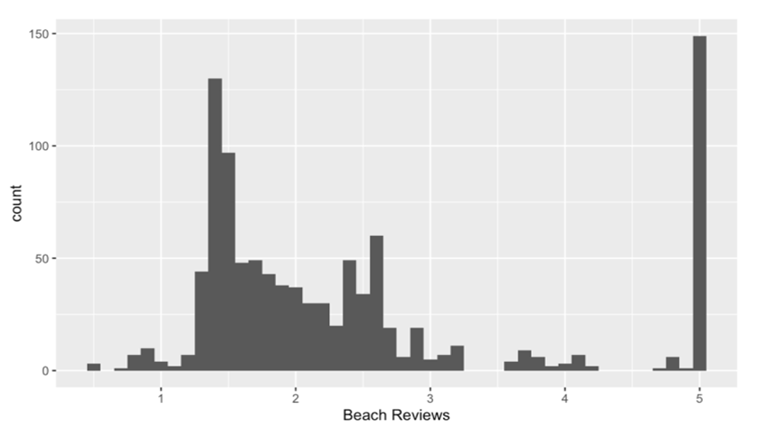 | Figure 1. Beach Reviews |
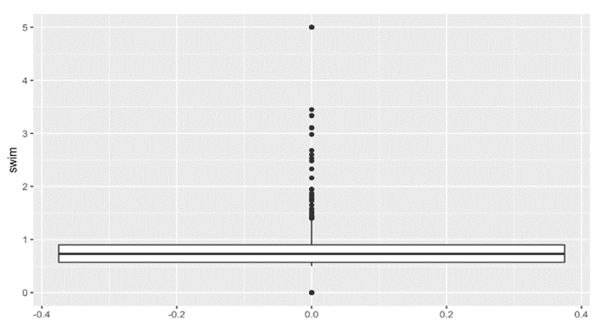 | Figure 2. Median review for swimming pools |
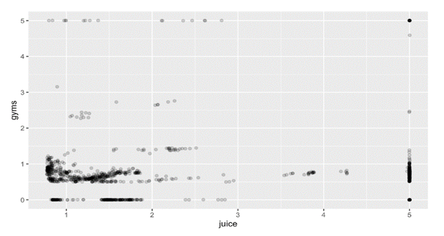 | Figure 3. Scatter plot Juice vs. Gyms |
2.2. Unsupervised Learning Methods
- The use of unsupervised learning methods was the cornerstone of the analysis, and a variety of methods were employed. Principal component analysis (PCA) was used to understand the structure of the data, while hierarchical and k-means clustering were used to examine and classify the different traveler archetypes. Each methodology revealed distinct insights about the data.
2.2.1. Principal Component Analysis
- Principal Component Analysis (PCA) is an unsupervised approach. Principal components allow us to summarize this set with a smaller number of representative variables that collectively explain most of the variability in the original set. PCA finds a low-dimensional representation of a data set that contains as much as possible of the variation. The idea is that each of the
 observations live in
  -dimensional space, but not all of these dimensions are equally interesting. PCA seeks a small number of dimensions that are as interesting as possible, where the concept of interesting is measured by the amount that the observations vary along each dimension. Each of the dimensions found by PCA is a linear combination of the
  features. The first principal component of a set of features
  is the normalized linear combination of the features
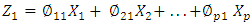 | (1) |
 We refer to the elements
  as the loadings of the first principal loading
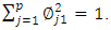
 We constrain the loadings so that their sum of squares is equal to one, since otherwise setting these elements to be arbitrarily large in absolute value could result in an arbitrarily large variance. Given a
  data set
  , how do we compute the first principal component? Since we are only interested in variance, we assume that each of the variables in X has been centered to have mean zero (that is, the column means of X are zero). We then look for the linear combination of the sample feature values of the form
 | (2) |
 After the first principal component
  of the features has been determined, we can find the second principal component
  . The second principal component is the linear combination of
  that has maximal variance out of all linear combinations that are uncorrelated with
  . The second principal component scores
  take the form
 | (3) |
 is the second principal component loading vector, with elements
  . It turns out that constraining
  to be uncorrelated with
  is equivalent to constraining the direction
  to be orthogonal (perpendicular) to the direction
  [12]However, the reviews are on a fixed scale of 0 to 5, and the exploratory analysis showed the variability was mostly homogenous across features indicating standardization was not necessary in this case. PCA was not used to construct traveler archetypes, but the insights were used in the clustering methods.
2.2.2. Hierarchical Clustering
- Agglomerative hierarchical clustering assigns observations in a dataset to a cluster based on how the observation is being linked to a cluster and the metric used to calculate the distance between the point and the cluster. Hierarchical clustering is a very flexible and customizable technique and allowed for the exploration of many methods to create traveler archetypes, and the different methods were evaluated using dendrograms.The following distance metrics were considered while using hierarchical clustering: Euclidean, Pearson, and Manhattan. Each distance metric has advantages and disadvantages. Euclidean distance operates as a quadratic penalty function, thereby generating very tight and distinct clusters that are geometrically “close”. Similarly, Manhattan distance calculates the absolute value of the distance between observations, and thus functions as a linear penalty function. Pearson distance considers the correlation between observations and is not a function of geometric proximity. Pearson distance will be small for vectors that are nearly parallel and large for vectors that are nearly orthogonal, regardless of their relationship in the data space. [13] In addition to the distance metrics, complete, average, and single linkages between observations were considered. since they have different operating characteristics. Complete linkage creates distinct and well-separated clusters by considering the distance between a new point and the furthest point in an existing cluster and thus can be considered a dissimilarity metric. The algorithm proceeds iteratively. Starting out at the bottom of the dendrogram, each of the
 observations is treated as its own cluster. The two clusters that are most similar to each other are then fused so that there now are
  clusters. Next the two clusters that are most similar to each other are fused again, so that there now are
  clusters. The algorithm proceeds in this fashion until all of the observations belong to one single cluster, and the dendrogram is complete.Single linkage creates sprawling, long-trailing clusters by considering the distance between a new point and the closest point in a cluster. Average linkage measures the average distance between a new point and all the points in a cluster and creates clusters that are more sprawling than complete linkage, but less long-tailed than single linkage.
2.2.3. K-means Clustering
- The second clustering method used was k-means. Unlike hierarchical clustering where the number of clusters is determined post hoc, the number of clusters to create using k-means is assigned a priori. [14]Additionally, the performance of k-means can be monitored through within-cluster sum-of-squares, giving the user an objective measure of accuracy. For these reasons, K-means was used to identify user archetypes and assign clusters for the supervised learning phase.
2.3. Supervised Learning Methods
- The identification of traveler archetypes has limited application for solving business problems. Correctly classifying individuals into the identified archetypes is critical for translating the data into actionable insights. To identify and classify Google users into traveler archetypes, a number of different supervised learning methods were investigated. These methods include Linear Discrimination Analysis (LDA), Quadratic Discrimination (QDA), K-Nearest Neighbors (KNN) and Tree-based Classification methods.
2.3.1. K-Nearest Neighbors
- K-NN is a widely used and high performing non-parametric classification algorithm. [15] The KNN classifier bases class predictions of an observation on k adjacent points. Adjacency—or nearness—is computed most commonly as Euclidean distance. A majority vote of the k neighbors is then used to assign the class. Much like PCA, hierarchical clustering, and k-means, k-NN is sensitive to the scale of the data. Any variables that are on a relatively larger scale will have a greater effect on the distance between the observations, and hence on the KNN classifier, than variables that are on a small scale. K-NN was anticipated to perform the best out of all supervised learning methods due to its similarity to the unsupervised methods used to determine traveler archetypes.
2.3.2. Linear Discriminant Analysis
- LDA models the distribution of the predictors separately in each of the response classes, and then uses Bayes’ theorem to flip them around into estimates. For more than one predictor, the LDA classifier assumes that the observations in the
 th class are drawn from a multivariate gaussian distribution which has a class specific mean and common variance. Class means and common variance must be estimated from the data, and once obtained are then used to create linear decision boundaries in the data. LDA then simply classifies an observation according to the region in which it is located. [16]When there are more than two classes, it is no longer possible to use a single linear discriminant score to separate the classes. The simplest procedure is to calculate a linear discriminant for each class, this discriminant being just the logarithm of the estimated probability density function for the appropriate class, with constant terms dropped. Sample values are substituted for population values where these are unknown. Where the prior class proportions are unknown, they would be estimated by the relative frequencies in the training set. Similarly, the sample means and pooled covariance matrix are substituted for the population means and covariance matrix.Suppose the prior probability of class
  is
is  , and that
  is the probability density of
  in class
  , and is the normal density equation.
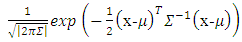 | (4) |
 and attribute
  is
is  and the logarithm of the probability of observing class
  and attribute
  is,
is,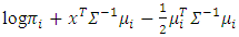 | (5) |
 are given by the coefficients of x.
  | (6) |
 by,
by,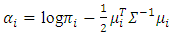 | (7) |
 and
and  . To obtain the corresponding “plug-in” formulae, substitute the corresponding sample estimators: S for
  for
for  ; and
; and  for
for  , where
  is the sample proportion of class
  examples. [17]
2.3.3. Quadratic Discriminant Analysis
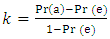
- QDA is very similar to LDA but does not assume constant variance across classes. Heterogenous class variances change the decision boundaries from a linear to quadratic, thus changing the behavior of the classifier. However, this additional complexity comes at cost. LDA is a simpler model with higher bias but less variation. QDA is a more flexible model that has lower bias but higher variance. LDA will outperform QDA when the decreases in bias are outweighed by the increases in variance.The quadratic discriminant function is most simply defined as the logarithm of the appropriate probability density function, so that one quadratic discriminant is calculated for each class. The procedure used is to take the logarithm of the probability density function and to substitute the sample means and covariance matrices in place of the population values, giving the so-called “plug-in” estimates. Taking the logarithm of Equation (4), and allowing for differing prior class probabilities
 we obtain
 | (8) |
 . Here it is understood that the suffix
  refers to the sample of values from class
  .In classification, the quadratic discriminant is calculated for each class and the class with the largest discriminant is chosen. To find the a posteriori class probability explicitly, the exponential is taken of the discriminant and the resulting quantities normalized to sum to unity. Thus, the posterior class probabilities
  are given by,
 | (9) |
 and associated expected costs explicitly. The most frequent problem with quadratic discriminants is caused when some attribute has zero variance in one class, for then the covariance matrix cannot be inverted. One way of avoiding this problem is to and a small positive constant term to the diagonal terms in the covariance matrix (this corresponds to adding random noise to the attributes). Another way, adopted in our own implementation, is to use some combination of the class covariance and the pooled covariance.Once again, the above formulae are stated in terms of the unknown population parameters
  , and
, and  and
and  . To obtain the corresponding “plug-in” formulae, substitute the corresponding sample estimators:
  for
for  for
for  ; and
; and  for
for  where
where  is the sample proportion of class
  examples. [18] [19]
2.4. Tree-based Methods
- Classification trees are a highly flexible statistical learning method that can capture non-linearities and interactions present in the data. Tree based methods begin by constructing decision trees through binary recursive splitting of the data. At each split, a cut point is chosen to minimize the heterogeneity of the resulting nodes. Single decision trees are notorious for relatively poor performance. Two methods—bagging and random forests—were used to improve the performance of tree-based methods in this paper.
2.4.1. Bagging
- Bootstrap aggregation, or bagging, is a general-purpose procedure for increasing the performance of a machine learning algorithm. Bagging involves bootstrap sampling training datasets from the original dataset, fitting the statistical learning methods, and aggregating the predictions appropriately. For this work, bagging was used on classification trees, so a majority vote of the predicted classes from the fitted trees was used as the prediction. [15]
2.4.2. Random Forests
- Bagging can be sensitive to strong predictors that repeatedly result in the sample split regardless of the bootstrap sample, which can lead to highly correlated trees and poor performance. Random forests remedy this situation by taking a random sample of the predictors at each point. Many trees are fit on bootstrapped samples and predictions are aggregated across all the models, very similar to bagging. The result is a collection of uncorrelated trees, and random forests often perform better than bagged trees. [15] [20]
2.5. Cross Validation (CV)
- Cross validation [15] was used to estimate the test accuracy rate of each supervised learning model. CV involves randomly dividing the set of observations into
 “folds” of approximately equal size. The first fold is treated as a validation set, and the model is trained on the remaining
  folds of data. This trained model is then used to predict the target in the Kth fold, and an accuracy metric,
  , is computed. This procedure is repeated
  times where a new validation set is used during each iteration. This process results in
  estimates of the test error:
  . The
. The  fold CV estimate is computed by averaging these values,
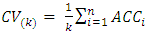 | (10) |
2.6. Kappa Statistic
- Accuracy can be a misleading metric since it is possible to make correct classifications simply by chance alone. Kappa was the preferred accuracy metric for this article, since it statistic adjusts accuracy by accounting for the possibility of a correct prediction by “guessing”. The following is the formula for calculating the kappa statistic:
 | (11) |
 refers to the proportion of actual agreement and
  refers the probability of making a correct classification purely by chance. Kappa values range from 0 to a maximum of 1 with a value of 1 indicates perfect agreement, a value of 0 indicating no agreement, and values between 0 and 1 indicating varying degrees of agreement. Depending on how a model is to be used, the interpretation of the kappa statistic might vary. Values above 0.8 were considered acceptable for this project. Traditional metrics such as precision, recall, and specificity can still be calculated with multiple classes, but the objective of this analysis was overall accuracy, not a specific error rate. [15] [21]
3. Results (Classes Assigned, Accuracy, Kappa)
- Results are divided into two parts. First, the constructed traveler archetypes are discussed. Second, the results from the supervised learning methods are presented.
3.1. Traveler Archetypes
- Figure 4 shows a biplot of the two first principal components of the unstandardized reviews dataset with an overlay of the original feature vectors. Four or five distinct groups of the original data vectors can be seen in the plot.A summary of the average values for each of the five classes assigned by the k-means algorithm is presented in Table 1. Some variables have a wide diversity across classes, while others have less separation. For example, the average rating for zoos is similar across classes, whereas restaurants have a wide dispersion across classes. Similarly, Figure 4 shows a biplot of the first two principal components colored by class assigned by k-means. The five groups of vectors seen in Figure 5 have their own associated class, demonstrating the structure identified during PCA was reinforced by k-means clustering.
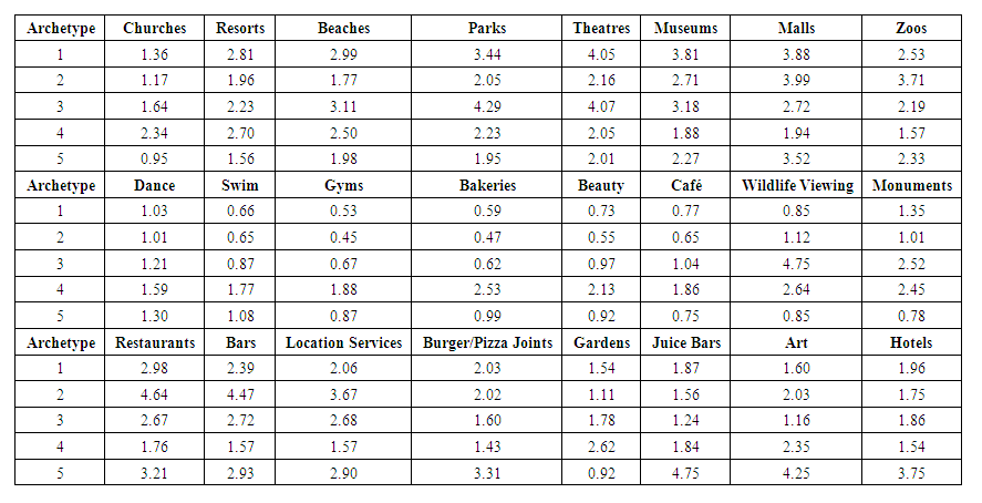 | Table 1. Average Archetype Values |
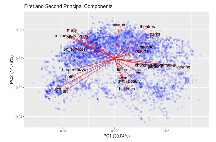 | Figure 4. Biplot of First and Second Principal Components |
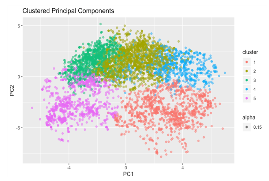 | Figure 5. PCA and Clusters |
|
3.2. Predicting Archetypes
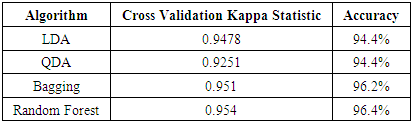
- K-nearest neighbors was the first statistical learning technique used. Figure 6 shows different values of the Kappa statistic for different values of K. The optimal number of neighbors is 229 achieving a kappa statistic of approximately 95%. This is an extraordinary level of accuracy for a classification algorithm and does not bode well for the success of the problem.
 | Figure 6. K-NN Performance for Different Values of K |
|
4. Discussions
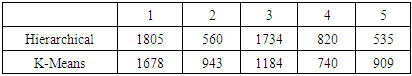
- The success of this research relies on correctly identifying the archetype structure in the data. Alignment between PCA, hierarchical, and k-means clustering suggests the methods employed approximate the true structure. Many different clustering methodologies were used to obtain classifications with similar results. Additionally, different numbers of groups were also tested without a change in the accuracy metrics. However, the accuracy rates of the supervised learning methods present several questions about the integrity of the results. It is highly unlikely to obtain an accuracy rate above 90%, and even less likely for all tested methods to have a similar level of performance. For these reasons, the authors are skeptical that the identified traveler archetypes are robust. Additional clustering methods could be employed to test the robustness of the conclusions, but this is beyond the scope of the paper. The classes identified above should be check by a domain expert for reasonableness. Since this in unlabeled data, it is not possible to test the model on new data. Ultimately, this model could be deployed on a small subset of customers and data could be collected on the performance of business metrics. For example, the models discussed above could be used to recommend advertisements for one group and click-through rates could be compared to a similarly sized control group. This could be a robust methodology to validate the models.
5. Conclusions
- Identifying consumer subgroups is essential for revenue optimization at large organizations. PCA was used to understand the underlying structure of the Google travel reviews dataset. Hierarchical and k-means clustering were used to identify consumer archetypes. K-NN, LDA, QDA, and tree-based methods were used to predict traveler classes. All supervised statistical learning methods performed extremely well; however, it is unlikely the assigned classes are correct. The models should be evaluated via an A/B test before putting them into full production.