-
Paper Information
- Paper Submission
-
Journal Information
- About This Journal
- Editorial Board
- Current Issue
- Archive
- Author Guidelines
- Contact Us
International Journal of Statistics and Applications
p-ISSN: 2168-5193 e-ISSN: 2168-5215
2021; 11(2): 37-49
doi:10.5923/j.statistics.20211102.03
Received: Jul. 20, 2021; Accepted: Aug. 6, 2021; Published: Aug. 15, 2021

Analysis of Balanced Random Survival Forest Using Different Splitting Rules: Application on Child Mortality
 Abstract
 Reference
 Full-Text PDF
 Full-text HTML
Hellen Wanjiru Waititu1, Joseph K. Arap Koske1, Nelson Owuor Onyango2
1School of Physical and Biological Sciences, Moi University, Eldoret, Kenya
2School of Mathematics, University of Nairobi, Nairobi, Kenya
Correspondence to: Hellen Wanjiru Waititu, School of Physical and Biological Sciences, Moi University, Eldoret, Kenya.
| Email: |  |
Copyright © 2021 The Author(s). Published by Scientific & Academic Publishing.
This work is licensed under the Creative Commons Attribution International License (CC BY).
http://creativecommons.org/licenses/by/4.0/

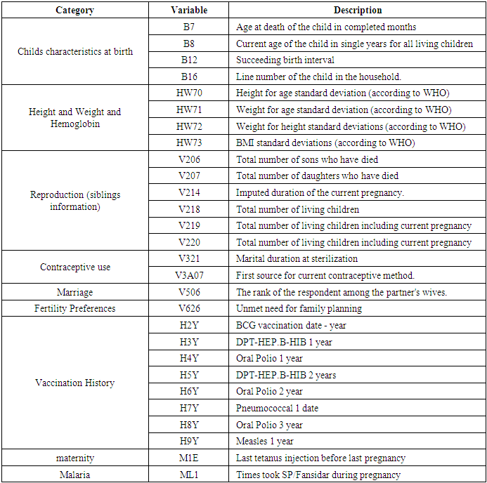
Under Five Child Mortality (U5CM) remains a major health problem in the developing world. The Sustainable Development Goals target of 25 deaths per 1000 live births has not yet been achieved in many Low and Middle Income Countries (LMIC). This study used the Kenya Demographic and Health Survey (KDHS) data (2014) to understand the determinants of U5CM. KDHS (2014) data is characterized by high dimensionality, high imbalance and violation of Proportional Hazard (PH) assumptions among other statistical challenges. This study aimed at handling the problem of non proportional hazard assumptions that characterize covariates of survival regression models. To achieve this we used various split rules, namely: log-rank, log-rank score and Bs.gradient splitting rules. The data used was balanced using Random Under-sampling method. The balanced data was integrated in RSF for variable selection while applying the three specified splitting rules. Respective selected variables were fitted in the Cox Aalen’s model for prediction while model selection was carried out using concordance index. The model with log-rank splitting rule recorded the highest concordance of 0.916 followed by Bs.gradient with a concordance of 0.864 while log-rank score resulted in a concordance of 0.799. In conclusion, the results from the analysis presented in this paper show the superiority of log-rank splitting rule. However, optimality of log-rank is achieved when the hazard is proportional over time. Some of the variables in the data were found to violate the PH assumption making the use of log-rank splitting rule not optimal. According to our analysis, we settle on Bs.gradient splitting method which still has a high concordance index of 0.86 and smaller error rate of 0.028. Using Balanced Random Survival Forests (BRSF) with Bs.gradient splitting rule, the identified determinants of U5CM are; V207 (sum of deceased daughters), V219 (sum total of living children) and B8 (age of the child). Hence, the age of the child and the siblings’ information are identified as some of the key determinants of U5CM.
Keywords: Splitting rules, Balanced Random Survival Forests, Under Five Child Mortality, Cox Aalen’s model
Cite this paper: Hellen Wanjiru Waititu, Joseph K. Arap Koske, Nelson Owuor Onyango, Analysis of Balanced Random Survival Forest Using Different Splitting Rules: Application on Child Mortality, International Journal of Statistics and Applications, Vol. 11 No. 2, 2021, pp. 37-49. doi: 10.5923/j.statistics.20211102.03.
Article Outline
1. Introduction
- In survival analysis, censored survival data are frequently predicted using semi-parametric methods. One of the most commonly used semi-parametric method in analysis of time to event data is the Cox Proportional Hazard (PH) method [1]. The Cox model estimates survival by evaluating various explanatory variables all at once. Other than being semi-parametric, Cox PH model is also popular due to its ability to produce adequately good regression coefficient estimates, survival curves and hazard ratios of interest for a wide variety of data occurrence [2]. However, the method makes assumptions which are not easily satisfied. One such assumption is that the hazard ratio between any two observations is proportional over time. In addition, Cox PH model does not take in to account the missing predictors, non-linearity of exponential factors and interdependence among observations.To deal with these limitations, nonparametric survival trees and forests have recently become useful alternatives. In 2008, [3] introduced Random Survival Forests (RSF), a fully non parametric ensemble tree based method for analysis of right censored survival data. The method can determine survival risk factors without assuming parametric associations. RSF generates a forest by randomly selecting a given number of bootstrap samples from the data in use. Each of the bootstrap samples develops into a tree through recursive partitioning of the covariate space. The trees then grow to full size until the end most node has no less than a predetermined number of exclusive events. RSF has the ability to discover non-linear effects, impute missing data and discover interactions beforehand.However, characteristic of survival data pose significant challenges to RSF. In this study, we worked with the 2014 Kenya Demographic and Health Survey (KDHS) data in trying to understand the determinants of Under Five Child Mortality. Some of the statistical challenges with the 2014 KDHS data include high dimensionality, high imbalance between mortality and non mortality classes and violation of Proportional Hazard (PH) assumptions among others. This study aimed at handling the problem of non proportional hazard assumptions that characterize covariates of survival regression models as well as dealing with high imbalance between mortality and non mortality classes. The aspect of high imbalance and violation of PH assumptions are often ignored by many researchers which can result to biased and inaccurate results.When working with highly imbalanced datasets, machine learning algorithms like RSF leads to biased results supporting the majority class. Additionally, highly imbalanced datasets poses significant challenges in RSF due to the stopping criterion which states that the terminal node should have no less than a predetermined number of unique events. This may result in premature termination of the tree especially when the mortality class is too small compared to the non mortality class. In 2020, [4] compared the performance of RSF in data balanced using different methods where random under-sampling method performed best in model selection using concordance index. In this paper, we used data balanced using random under-sampling method where the mortality and non mortality classes have equal number of observations.The problem of variables violating PH assumptions has often been ignored by many researchers. Some survival analysis methods such as the Cox PH models apply the restriction of satisfaction of PH assumption. During node splitting process in RSF, the most commonly used splitting rule is log-rank test. The optimality of log-rank test is achieved when the hazards are proportional over time. Proportional hazard (PH) assumption indicates that the effect of covariate is the same at all points. However this is usually not the case since in many instances, variables violate the PH assumption making the use of log-rank test and Cox PH model among others not optimal.In some cases, researchers ignore this assumption leading to inaccurate conclusions. Others delete variables that violate the PH assumption in order to work with the restricting methods. However, the deleted variables could be important predictors of mortality. There is need to therefore work with methods that take into consideration these statistical challenges.Quite a number of studies have researched on splitting rules used in RSF. These include [5] who proposed an improved RSF by using weighted log-rank test in splitting the node while using the model of [6]. [7] In 2018 used R-squared splitting rule in survival forests, [8] compared RSF using different splitting rules among others. [9], [10], [11], [12] and [13] among others used Log-rank test for survival splitting as a measure for maximizing survival difference between nodes. In this research, we analyze the performance of BRSF using different splitting rules while using data balanced using under-sampling method. This was done using 2014 KDHS data in identification of determinants of Under Five Child Mortality (U5CM).The rest of the paper is laid out as follows: Section 2 discusses the methodology employed in this study, from description of the data, exploration of PH assumption, the theory behind RSF and node splitting, the different splitting methods used, survival tree estimators, effect of predictors using Cox Aalen’s model and finally model selection criteria using concordance statistic. Section 3 summarizes the results of the study with respect application of RSF, variable selection using RSF with the different splitting methods and model selection using concordance statistic. Finally, section 4 offers a discussion of our results against other ongoing research.
2. Methodology
2.1. Data Description and Management
- The data used in this research was obtained from the 2014 Kenya Demographic and Health Survey (KDHS) data [14]. KDHS is a national proceeding which is carried out every five years in the country all the way back from 1989. Thus, 2014 KDHS is the 6th Demographic and Health Survey (DHS) operation in Kenya. The survey is headed up by the Kenya National Bureau of Statistics (KNBS) which is the leading Government agency for official statistics in collaboration with the National Council for Population Development, Ministry of Health, and a number of development partners. Their aim is to collect data required for health, nutrition, planning, monitoring and evaluation of population among others. 2014 KDHS is a sample survey data in which households are randomly chosen from the KNBS sampling frame. The units of analysis in this data are household, individual, children aged o to 5 years, woman aged 15 to 49 years and man aged 15 to 54 years.After successful application and acquisition of the 2014 KDHS data, it was downloaded and viewed using Statistical Package for Social Sciences (SPSS). The overall data had 1099 variables and 20994 observations. From the overall data, variable with 100% missing observations and others which were highly correlated were deleted. At the same time, status and time variables which are of great importance in survival data were calculated and included in the data. Time from birth to date of interview was taken as the follow-up period. This resulted to a total of 786 variables while the observations remained at 20964. The data was found to be highly imbalanced with the mortality class taking 4% of the data as seen in [4]. Various covariates were similarly found to be highly imbalanced resulting to a range of 3-6% of the mortality class.The data was categorized into regions which are equivalent to the former provinces in Kenya. Since our interest was to deal with a relatively smaller sized data, we analyzed data from Nairobi region which is a unique urban setting with diverse levels of social economic status among populations. The Nairobi region data consisted of 532 observations and 757 variables. This was after removal of variables with 100% missing observations in the region. Other variables like region, residence, county which had similar response in the region were also deleted from the data. Nairobi region dataset was similarly highly imbalance. The mortality class representation in this region was 6.4% while the range of mortality representation in the covariates was 0-7% as seen in our previous work, [4]. Data balancing was performed using 4 methods. Model selection using concordance index showed good performance in random under-sampling method followed by synthetic minority oversampling technique (SMOTE). In this paper, we analyze the performance of the under-sampled dataset using RSF with different splitting rules. The dataset is fully balanced after random under-sampling with each class taking half of the sample size. The balanced dataset had a total of 68 observations with the mortality and censored classes each having 34 observations which represent 50% of the sample. The number of variables in the dataset was 757.
2.2. Proportional Hazard (PH) Assumption
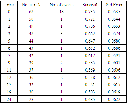
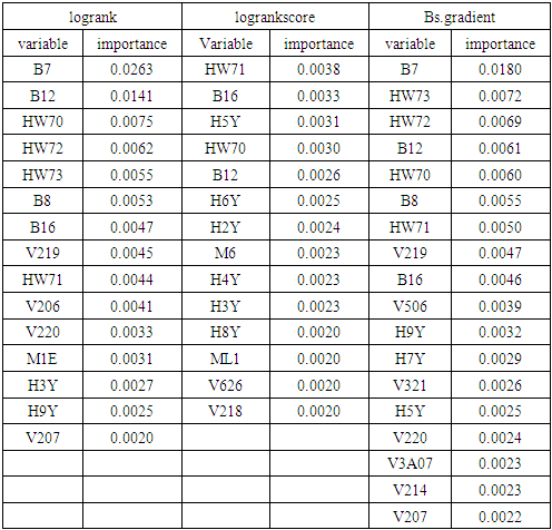
- Hazard is the likelihood of an event happening at any given time point given that the event had not occurred. The PH assumption indicates that the ratio of the hazard comparing any two specifications of covariates is unchanging or proportional over time. It is essential to verify whether the predictor variables in the model satisfy the PH assumptions. We used Kaplan Meier curves to explore the PH situation.The Kaplan Meier curves plots the estimated proportion at risk (survival probability) against time giving the estimated survival functions [15]. The curves are in form of step functions with each vertical drop pointing out one or more deaths happening [16]. If the variables satisfy PH assumption, the survival curves should be parallel. If for two or more categories of a variable of interest do not result to parallel curves or the curves cross, then it is an indication that the PH assumption is violated. Before the exploration of PH assumption, we got the general view of the survival data by demonstrating the occurrence of event during the follow-up period as shown in table 1 and the survival curve in figure 1.
|
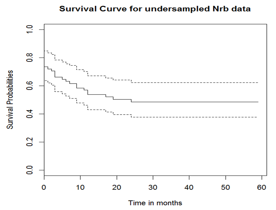 | Figure 1. General survival curves for the data used |
2.3. Exploration of Proportional Hazard
- The aspect of hazard being constant over time was explored using Kaplan Meir curves. Figure 2 shows Kaplan Meir curves for some of the covariates.From the survival curves in figure 2, there is evidence of violation of PH assumption by some of the covariates as demonstrated by the presence of crossing curves. Survival curves by child sex are almost parallel with female children having a higher survival probability throughout the period than the male children. The two curves do not cross but they are not perfectly parallel. From survival curve by level of education, there exist individuals with no education but none of them got an event. Hence the horizontal blue line with survival probability of 1. Crossing curves are observed between secondary level and higher education level showing violation of PH assumption. The survival probability for the secondary education category is higher than that of higher level from 0 to about 12 months when the curves cross. From 12 to about 25 months, individuals in higher level show a higher survival probability than those in secondary level. Individuals with primary level of education are observed to have a higher survival probability than those in secondary and higher education level. Similarly, survival curve by wealth index indicate violation of PH assumption since the curves for poorer and middle level categories are crossing.
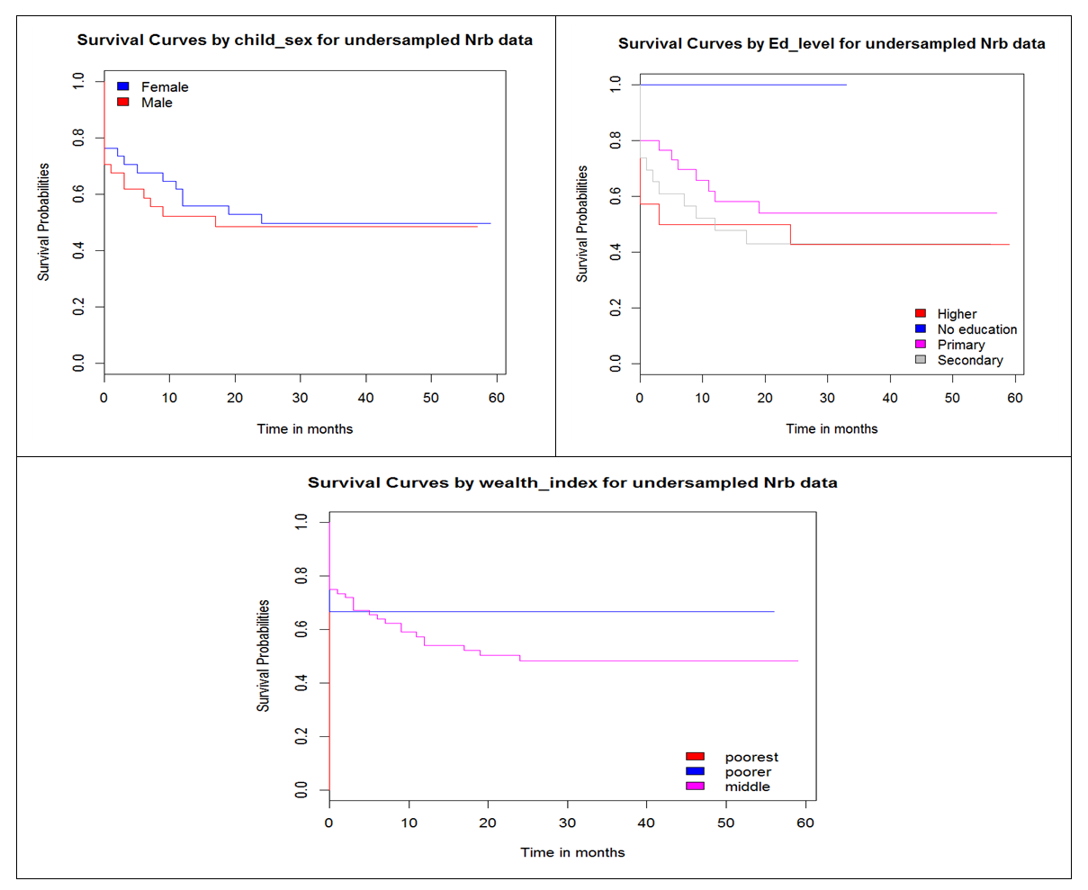 | Figure 2. Survival curves by covariates |
2.4. RSF Algorithm for Variable Selection
- The balanced data was integrated with RSF algorithm which is described by [3] as follows:a) The process starts by drawing at random
 bootstrap samples from the original data having
  samples. On average, each bootstrap sample sets aside 37% of the data named as Out of Bag (OOB) data with respect to the bootstrap sample and each sample has
  predictors.b) For each bootstrapped sample, a survival tree is developed. This is done by randomly choosing
  out of
  variables in
  for splitting on. The value of
  depends on the number of available predictors and is data specific. All the
  bootstrap samples are designated to the top most node of the tree which is also referred to as the root node. This root node is then separated into two daughter nodes each of which is recursively split progressively maximizing survival difference between daughter nodes.c) The trees are grown to full size where the end is indicated by the restriction that the endmost node should have larger than or equal to
  unique events.d) After the tree is fully grown, the in-bag and out of bag (OOB) ensemble estimators are computed by taking the mean value over all the trees predictors.e) The ensemble OOB error is calculated using the first
  trees, where
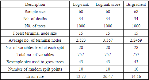
  .f) OOB estimation is used to calculate the Variable Importance (VIMP) [17].By averaging over all trees, a reliable measure of importance of a variable regarding time to event can be obtained [18].RSF gives a measure of VIMP which is totally nonparametric. VIMP has been found to be effective in many applied settings for selecting variables [19], [20], [21], [22], [23]. In this study, using the RSF model, the highly predictive risk factors using three different splitting rules were extracted.
 2.4.1. Splitting the Node in RSF
- Time and status variables are of great importance in survival data. The time variable indicates the survival duration while status variable indicates whether the observation experienced an event or was censored. The actual survival time of censored observation cannot be calculated since censored observations do not terminate. The only indication of known survival duration is the occurrence of an event. The presence of censoring in survival data complicates certain aspects of implementing RSF [17]. While taking into account right censoring, the observed data is given in the form
 where
where  is defined as the minimum of the event and censoring time. Hence
  where
where  is the event time and
  the censoring time.
  is the censoring indicator defined as
  .While growing a tree in RSF, node splitting must take censoring into consideration. With reference to the RSF algorithm, a forest develops from randomly drawn
  bootstrap samples each of which becomes the root of each tree in the forest. There being
  predictors in each bootstrap sample,
  predictors are randomly chosen for splitting on. Suppose we take
  to be the top most node of the tree which is to be split into two daughter nodes. Within the node, there exist
  predictors and
  observations. The splitting process is as follows [24]. • Take any predictor
  from the
  predictors.• Find the splitting value
  such that the survival difference between
  and
and  for predictor
  is maximum. In this case
  splits to the left daughter node while
  splits to the right daughter node.• Calculate the survival difference between the two daughter nodes using a pre-determined splitting method.• Take another split value
  in predictor
  until we get a split value which results in maximum survival difference for predictor
  .• From the remaining
  predictors in the node the process is repeated until we get predictor
  and split value
  which give maximum survival difference between the two daughter nodes.• Applying the node splitting process in each of the new daughter nodes and recursively partitioning the nodes leads to the growth of the tree.• The process is applied to all the
  root nodes leading to the growth the forest.When survival difference is maximum, unlike cases with respect to survival are pushed apart by the tree. Increase in the number of nodes causes dissimilar cases to separate more. This results in homogeneous nodes in the tree consisting of cases with similar survival. In this research, the following splitting methods were used to calculate the survival difference between any two daughter nodes.
2.4.2. Log-Rank Splitting Rule
- Log-rank splitting rule separates the nodes by selecting the split that yields the largest log-rank test. The log-rank test is the most frequently used statistical test to compare two or more samples non-parametrically in censored data. PH assumption is the key requirement for the optimality of log rank test. Suppose we want to split node
 of a tree using log-rank splitting rule. The data at the node is presented as
  where
where  is the
  predictor,
  and
and  represent the
  survival duration and censoring status respectively. The information at time
  can be summarized as in the table below.
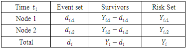 Where,
  stands for the number of events in daughter node
  at time
 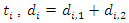 .
. represent individuals who are alive in daughter node j,
  at time
  is the number of
 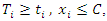 where
where  is the duration of survival for the
  individual and
  the distinct event time in node
 is the number of
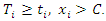
 For a split using covariate
  and its splitting value
  The survival difference between any two daughter nodes is calculated using log-rank test given as;
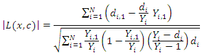 This equation measures the magnitude of separation between two daughter nodes. The best split is given by the greatest difference between the two daughter nodes which is given by the largest value of
  [25].
[25].2.4.3. Log-Rank Score Splitting Rule
- Log-rank score splitting rule [26] was developed from log-rank split rule. The ranks for each survival time
 are computed given an ordered predictor
  such that
 The rank for each time
  is calculated as
 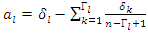 where
where  the number of
  . Let
. Let  and
and  be the sample mean and sample variance for
  for
for  The formula for log-rank score test is given by
 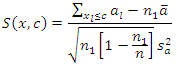 This split rule gives the magnitude of node separation by
  where the best split is given by the maximum value over
  and
and 
2.4.4. Gradient-Based Brier Score (Bs. Gradient) Splitting Rule
- Brier Score (BS) is the most frequently used scalar summary of correctness for probability predictions for binary events. Let
 be the
  likelihood prediction in a series of
  such predictions. The paired observation is given as
  if the event of interest occurs on the
  occasion, and
  otherwise. The BS is the mean-squared error over the
  pairs of prediction observations,
 In this case, the time horizon used for the Brier score is set to the
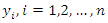
  percentile of the observed event times which must be a value between 0 and 1. Suppose we have a pair of predictor-response, say
  for
for  . The usual regression procedure attaches the conditional average of the response variable
  to a specified set of predictors
  [27] introduced Quantile Regression Forests (QRF) which connects between an empirical cumulative distribution function and the outputs of a tree. Let
  be a group of randomly selected variables to be split into two daughter nodes
  and
and  . Suppose the homogeneity of each group is defined by
  where
where  is the sample mean in
  For an optimal splitting selection, comparison is done between the homogeneities of
  and
and  with that of
  . The splitting value
  is the one that maximizes
  Where
Where  is a randomly selected sample of predictors from the predictor space
  . The resulting nodes are recursively split until the stopping criterion is reached. The terminal node gives the predicted value. [28] Suggested that instead of maximizing variance heterogeneity of the daughter nodes, one maximizes the criterion
  where
where 
 is an indicator function which takes a value of 1 when
  is more than the
  quantile
  of the observations of node
  The selection of
  is connected with a gradient based approximation of the quantile function
 , hence the term gradient forest. The order for each split is chosen among given orders
  .
. 2.5. Survival Tree Estimators
- In RSF, the tree growing process begins by randomly selecting
 bootstrap samples from the original data. Each bootsrap sample sets aside on average 37% of the data called
  data while the remaining 63% is called the in-bag data. The in-bag data is used to grow the tree and gives estimators which are used for prediction. On the other hand, the
  data is not involved in the growth of the tree but used for cross-validation purposes. RSF estimates cumulative hazard function (CHF) and survival function based on the terminal nodes using the in-bag and out-of-bag estimators.
2.5.1. In-Bag Estimators
- Let:
 denote the terminal node of a tree.
 Indicate the distinct event times within node h,
 Indicate the number of deaths at time
  and
and Indicate the number of individuals at risk at time
  The CHF for node
  is approximated using the bootstrapped Nelson–Aalen estimators;
 This implies that for a given tree, the hazard estimate for node
  is the ratio of events to individuals at risk summed across all unique event times. Each terminal node of a tree provides a sequence of such estimates and each individual in node
  has the same CHF.The survival function for node
  is estimated using bootstrapped Kaplan Meier estimator;
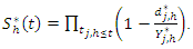 This gives the estimates for the individuals in node
  at a given time
  To estimate the CHF for a given predictor
 and the survival function of a given predictor
 is dropped down the tree and ends up in a distinct endmost node as a result of the binary nature of the tree. This implies that
  and
and  .This defines the CHF and survival function for all individuals in the data and the estimates for the tree. Due to bootstrapping (sampling with replacement) an observation can be found in various bootstrap samples and hence in various trees.The in-bag ensemble estimators are computed by averaging the trees estimators. Hence the in-bag ensemble CHF and survival estimators are respectively given as
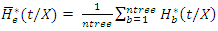 and
and 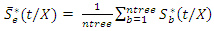
2.5.2. Out-Of-Bag (OOB) Estimators
- Let
 be an indicator pointing to whether case
  is in-bag or out of bag such that
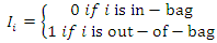 To determine the CHF and survival estimators for an
  case
case  , the case is dropped down the tree to a endmost node
  . The OOB CHF and survival estimators for
  becomes
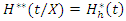 and
and 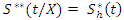 respectively.The OOB ensemble estimators are calculated by getting the mean of the OOB tree estimators. Hence the OOB ensemble estimators are given as
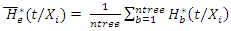 and
and 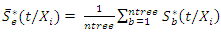
2.6. Determining the Variable Effects
- RSF gives a measure of Variable Importance (VIMP) which is totally nonparametric. In this study, the highly predictive risk factors from the balanced dataset were extracted using the RSF model. The extracted important predictors were then examined for PH assumption satisfaction. This was done by examining scaled Schoenfeld residuals and use of statistical tests shown in table 4. Since the PH assumption did not hold for all the variables, we took into consideration analyses that take into account time-varying effects. Cox-Aalen’s model proposed by [29] is one of the tools for handling the problem of non-proportional effects in the variables. The model provides a way of including time-varying covariate effects. In a datasets where some of the covariates effects are constant while others are not constant, Cox-Aalen’s model is a better alternative since it combines the two types of covariates. In the model, the covariates are subdivided into two parts in which one part act additively on the intensity while the other work multiplicatively. The Cox Aalen’s model is defined by,
 where,
 is the indicator of the risk.
  is a
is a  vector of covariates where
  is the additive non parametric time varying covariate and
  are the covariates with constant multiplicative effects.
  Is a
Is a  vector of time varying regression coefficients and
  is a
is a  vector of relative risk regression coefficients.Comparison of prediction accuracy of the different models was done based on concordance index.
3. Results
3.1. Variable Selection Using BRSF with Different Splitting Rules
|
|
3.2. Results of Test for PH Assumption
- PH assumptions that the relative risks are constant over time were tested by examining scaled Schoenfeld residuals as shown in figure 3 and use of statistical tests shown in table 4.
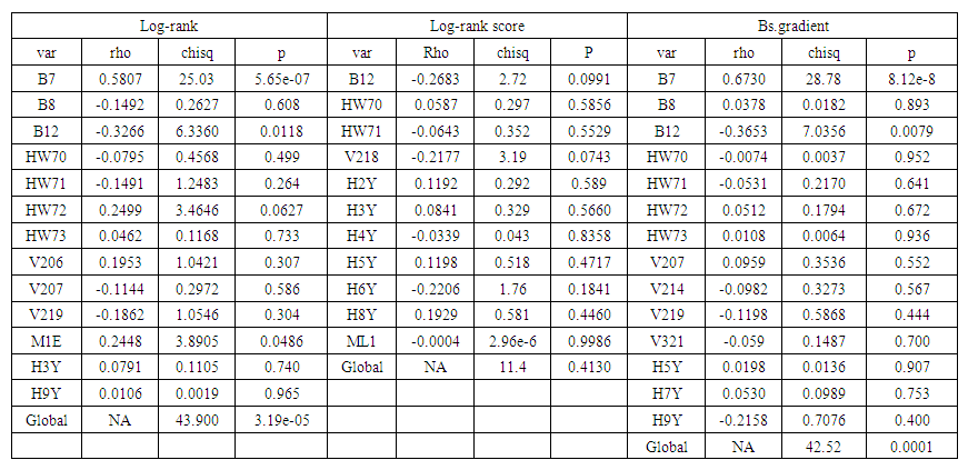 | Table 4. Statistical Tests (Test for PH assumption). PH assumption is supported by non significant P-values |
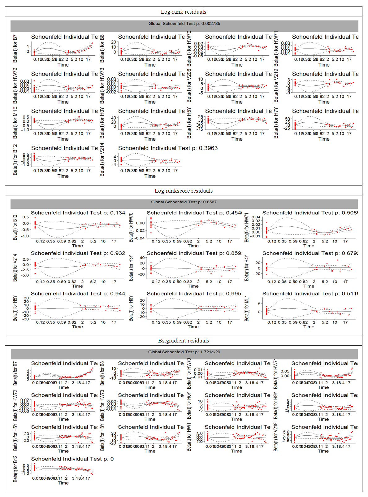 | Figure 3. Schoenfeld residuals |
3.3. Results of Prediction Using Cox Aalen’s Model
|
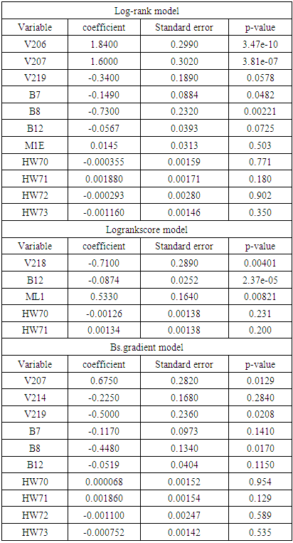
 ) are V206, V207, B7, and B8 from the log-rank model, V207, V219, and B8 from the Bs.gradient model and V218, B12 and ML1 in the log-rank score model. To compare the different models, concordance index was used in order to determine the effect of the various splitting methods and results shown in table 6.
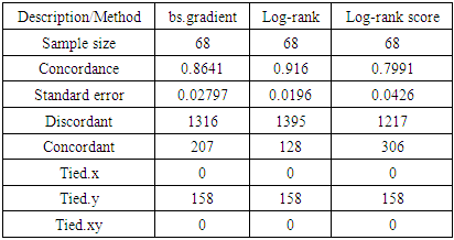
 3.4. Results of Model Selection
|
4. Discussion
- In this study, we analyzed the performance of data balanced using random under-sampling method under different splitting rules. The study addressed the challenges of data balancing and violation of PH assumptions. The splitting rules used are the log-rank, log-rank score and BS.gradient splitting rules. The performance was based on 757 variables in prediction of Under Five Child Mortality from the 2014 KDHS data.From our findings, the model that used log-rank splitting rule performed best with the largest concordance index of 0.916 and smallest error rate of 0.019. This was followed by the model with Bs.gradient splitting rule with a concordance index of 0.864 and error rate of 0.028. Log-rank score had the smallest concordance index of 0.799 and highest error rate of 0.043. Other researchers have explored the issue of splitting rules in RSF. [31] Used four splitting rules (log-rank, log-rank approximation, log-rank score and conservation of events) in RSF where log-rank splitting rule performed best with the smallest error rate. Log-rank test has been used for survival splitting as a means of maximizing survival difference between nodes [9], [10], [11], [12], and [13] among others.Despite its good performance, use of log-rank splitting rule is not appropriate when the PH assumption is violated. From the 2014 KDHS data, some of the variables were found to violate PH assumption making the use of log-rank method not appropriate. A number of studies have explored on the different splitting rules in RSF. [5] Proposed an improved RSF by using weighted log-rank test in splitting the node while using the model of [6]. [7] Used R-squared splitting rule in survival forests while [8] compared RSF using different splitting rules. [32] Proposed Harrell’s Concordance index (C index) split criterion in RSF. In their research, they did a comparison between C index splitting rule with the log-rank splitting rule where C index splitting rule was found to perform better than log-rank when censoring rate is high and in smaller scale clinical studies.In this study, we have addressed the challenges of imbalance in the datasets and selection of the most optimal splitting method when PH assumption is violated. The challenge of high imbalance between mortality and non mortality class was addressed by working with data balanced using random under-sampling method before integrating the data with RSF. Studies that researched on use of balanced data in RSF includes [30] who developed a BRSF by integrating synthetic minority over-sampling technique in RSF and [4] who analyzed the performance of RSF using different balancing techniques (random under-sampling, random over-sampling, both-sampling and synthetic minority over-sampling technique), where random under-sampling emerged the best. In this study, we considered a balanced dataset for maximum growth of the trees. The BRSF was then analyzed using log-rank, log-rank score and Bs. Gradient splitting rules when the PH assumptions are violated where Bs.gradient splitting rules was found to be the most suitable splitting rule.
5. Conclusions
- In this paper, we have analyzed the performance of BRSF using different splitting rules. This addressed the challenges of imbalance which is commonly occurring in survival data and also selection of the most optimal splitting rule when PH assumption is violated. The results from the analysis presented in this paper show the superiority of log-rank splitting rule. However, optimality of log-rank is achieved when the hazard is proportional over time. It is clear from the survival curves by covariates shown in this paper as well as the statistical tests that most variables in the dataset used violate the PH assumption making log-rank not appropriate for node splitting. According to our analysis, we settle on Bs.gradient splitting method which still has a high concordance index of 0.86 and smaller error rate of 0.028. Use of balanced data and good choice of an optimal splitting rule that can separate high risk variables and low risk variables leads to further improvements in RSF. This brings about high levels of accuracy during prediction process. Using BRSF with Bs.gradient splitting rule, the identified determinants of U5CM are; V207 (sum of deceased daughters), V219 (sum total of living children) and B8 (age of the child). Hence, the age of the child and the siblings’ information are identified as key determinants of U5CM.