Ilaria L. Amerise
Dipartimento di Economia, Statistica e Finanza, Università della Calabria, Via Pietro Bucci, Cubo 1c, 87036 Rende (CS), Italy
Correspondence to: Ilaria L. Amerise, Dipartimento di Economia, Statistica e Finanza, Università della Calabria, Via Pietro Bucci, Cubo 1c, 87036 Rende (CS), Italy.
| Email: |  |
Copyright © 2021 The Author(s). Published by Scientific & Academic Publishing.
This work is licensed under the Creative Commons Attribution International License (CC BY).
http://creativecommons.org/licenses/by/4.0/

Abstract
Companies and public or private entities identify accurate and timely forecasts of tourism demand as a strategic objective that can increase both their global competitiveness and their market share. In this paper, the Reg-SARMA approach is used to build simultaneous prediction intervals for monthly tourist arrivals in Italy. A Reg-SARMA model is a multiple regression whose error component is assumed to follow a multiplicative SARMA process. A three-stage procedure is applied. First, we set up a multiple linear regression model including only deterministic explanatory variables to facilitate the construction of the prediction intervals. Then the parameters are estimated using ordinary least squares and the residuals captured to serve as a basis for the second stage. Here, a SARMA process is fit to the regression residuals. In the final stage, both the fitted residuals and the estimated errors act as additional regressors in an extended regression equation to be re-estimated using least squares. The advantage of this method is that the new regressors have eliminated any serial correlation between the original residuals. Application to Italian data shows that the proposed approach generates effective and efficient point and interval forecasts, which can be of help to tourism managers, marketers, planners and researchers.
Keywords:
Regression with time series errors, Simultaneous prediction intervals, Multiplicative seasonal ARMA models
Cite this paper: Ilaria L. Amerise, Forecasting Tourist Arrivals in Italy, International Journal of Statistics and Applications, Vol. 11 No. 2, 2021, pp. 28-36. doi: 10.5923/j.statistics.20211102.02.
1. Introduction
The perishable nature of the tourism product and the vulnerability of its market to a variety of external factors (e.g. complementary services, natural and human-made disasters) make the robustness and promptness of predictions essential to achieve substantial improvements in planning travel facilities. There are many ways to generate prediction, ranging in complexity and data requirements from intuitive judgement through time series analysis to multi-equation econometric models. Tourism arrival forecasting methods can be broadly divided into four categories: time series models, econometric models, artificial intelligence techniques and qualitative methods [1]. For a still reasonably up-to-date overview see [2].Forecasting is necessary, but it is at least as essential to providing an assessment of the uncertainty associated with forecasts from one step to  steps ahead, where
  is the prediction horizon of interest. An important method to assess the uncertainty consists of the formulation of a probabilistic statement about all
  forecasts simultaneously and not on one about each forecast separately. It should be evident that this topic focuses on forecast using embedded information in the time series data, which can be quite useful for planning purposes. However, they do not provide organizations with a model to assess their current situation against other organizations or to change, if necessary, the course of the future. See [3].The specific aim of this paper is to employ the Reg-SARMA method to forecast tourist arrivals to Italy. The procedure follows these steps:1. In the part “Reg”, arrivals are estimated using a multiple regression model with non-stochastic predictors.2. In the part “SARMA”, the regression residuals from the “Reg” component are analyzed by means of a Box-Jenkins process to ascertain whether they are random, or whether they exhibit patterns that can be used to improve fitting and enhance prediction accuracy.3. The two components are estimated separately and then combined together into a single equation at a later stage. 4. The final model will provide point and interval forecasts for future monthly occupancy in collective tourist accommodation establishments. The paper proceeds as follows. Section 2 outlines the construction of the classical linear regression model, which will be based on a standard set of hypotheses so that the only problem left is the selection of the explanatory variables. Section 3 discusses the choice of the SARMA process that best describes the behavior of the regression residuals estimated in the previous section. We consider a very broad class of processes and select the stationary and invertible process that yields the smaller Akaike information criterion. Then, the residuals in the original regression model are replaced by the fitted values of the best SARMA process. Finally, regression and SARMA parameters are re-estimated together using the ordinary least squares and taking advantage of the fact that the new regressors have eliminated any serial correlation between the original residuals. In Section 4 we present a general procedure for the construction of simultaneous prediction intervals for multiple forecasts generated by the Reg-SARMA model outlined in Section 3. Applications to the Italian data show that the proposed approach is not only effective in point forecasting of tourism arrivals, but also in constructing SPIs for multiple forecasts generated by a Reg-SARMA model, thus reducing the risk that a decision will fail to achieve desired objectives. Section 5 includes concluding remarks.
2. Regression Analysis
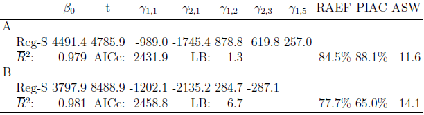
Regression models are used to examine the dependency among a given set of explanatory variables or predictors, one of which is specified as dependent. The relationships are expressed in the form of a linear equation relating the response or dependent variable and some explanatory variables. More important, models are often used to make statements about future values of the response variable for given values of the predictors. In our specific context, the response variable is the number of monthly arrivals to Italy from other parts of Italy and from other countries. The two time series span from January 2002 to August 2019. See [4]. Figure 1 shows the time series to be modelled.It is evident that the two series have a similar trend, but different levels and seasonalities in the middle of the year. It is also clear that, there is a decline of the arrivals in the last two years of the time series.
2.1. Building the Regression Model
In order to keep the estimation problem tractable, the predictors included in the regression model are all deterministic functions of time, meaning that we know their future values exactly. Such a choice is suggested by the fact that stochastic predictors are not under the control of the researcher and must also be forecast. According to [5], this is one of the possible causes of inefficiency in interval forecasting, which is our primary interest, in fact.After a series of preliminary experiments and literature review, we have restricted the choice of explanatory variables to two distinct sets. The first set intend to capture the trend-cycle component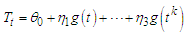 | (1) |
where 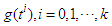 are orthogonal polynomials in
  of degree
  . The use of orthogonal polynomials results in uncorrelated regressors so that multi-collinearity cannot occur. We want relatively simple trends that capture broad movements in the dependent variable. The time series in Fig. 1, show a monotone trend and
  seems to be sufficient for describing the general course of both the time series.
 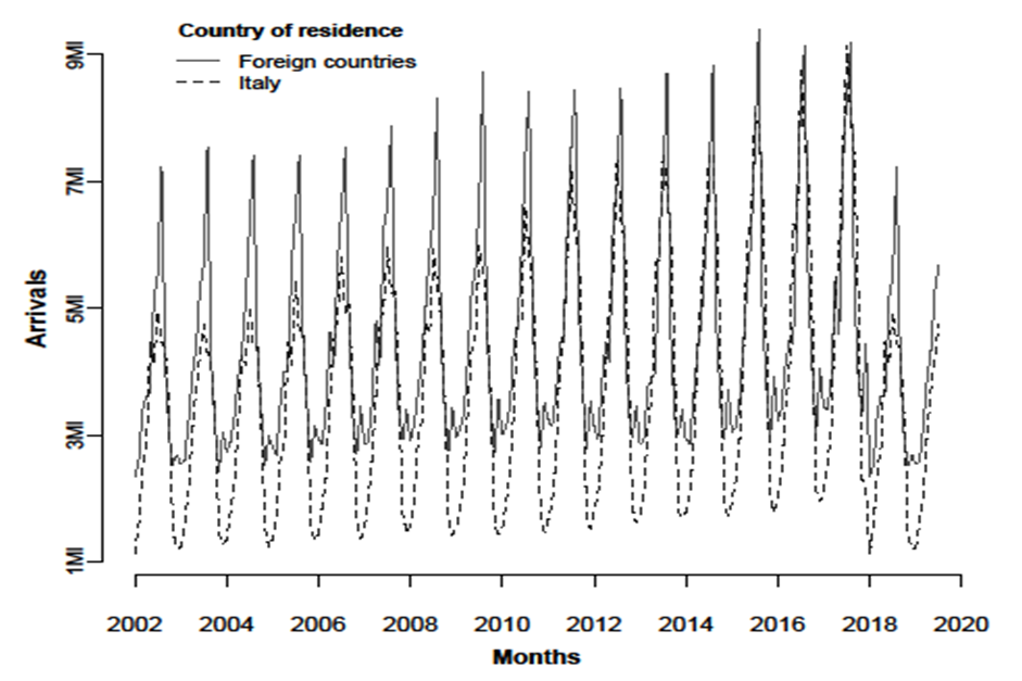 | Figure 1. Arrivals to Italy |
The second set of predictors comprises trigonometric functions of time, which are designed to reconstruct the seasonal component of the time series 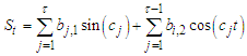 | (2) |
where  and
and  is the seasonal periodicity. Notice that, the last harmonic in the second expression is left incomplete to prevent perfect collinearity. To uncover the cycles in the arrivals we computed the periodogram as implemented in the
  package TSA [6]. The most pronounced periodicity is
  which will be the only seasonal pattern considered in the follow-up analysis. In summary, the regression equation for the relationship between tourist arrivals and time can be represented in the following form
 | (3) |
where  represents monthly tourist arrivals in the period from 1 to
  . Notation
  indicates a
  vector of predictors that include 4 parameters of the cubic trend and 11 harmonics depicting the monthly seasonality for a total of a total of
  parameters.The predictors are aggregated to form a
  design matrix
  with full rank
  and
and  . Finally,
  is a
is a  vector of unknown parameters which are to be estimated from observed data. We assume that
  so that the design matrix
  contains a column of ones and, without loss of generality, it will be assumed that the means of the other columns are all zero. We also assume that the error
  have a Gaussian distribution with zero mean and variance-covariance matrix
  where
where  is the identity matrix of order
  . Due to the high number of predictors, it is advisable to perform some sort of screening procedure with sequential strategies such as stepwise selection. To this end we carry out a preliminary, albeit schematic, selection based on stepwise backward elimination. The variables are sequentially discarded from the model one at a time until no more predictors can be removed. At each stage, the predictors are identified whose
  -value of the corresponding
  -statistic are higher than a prefixed threshold
  . The constant
  is the minimum level of significance to reject the hypothesis
  , that is,
  implies that the predictor
  is a candidate to be removed. The
  -values should not be taken too literally because we are in a multiple testing situation where we cannot assume independence between trials. Accordingly, we have established
  . If, at a given stage, there are more than one predictors verifying the condition
  , then the predictor which has the largest VIF (variance inflation factor) is canceled from the set. Removals continue until the candidate to exit has a
  -value lower than the minimum level
  .
.
2.2. OLS Estimation and Adequacy of Fitting
At this preliminary stage the parameter estimates are based on the ordinary least squares (OLS) | (4) |
The OLS estimate of the residual variance is given by | (5) |
Under the hypothesis of Gaussian residuals, vector  has a Gaussian distribution with mean vector
  and variance-covariance matrix given by
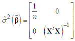 | (6) |
Moreover, the variable  has a
has a  distribution with
  degrees of freedom and it is independent of
  .The adequacy of fitting models is studied by using the values of the adjusted
  and the bias-corrected Akaike information criterion
 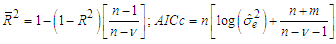 | (7) |
where  is the coefficient of multiple determination of the regression equation,
  is the number of unknown parameters of the model,
  and
and  is the estimated variance for the fitted regression. The two statistics move in two different directions. Models having a larger
  or a smaller
  are preferable. The OLS model presupposes the absence of serial correlation between residuals. If this is not true, then this fact can be detected through the auto-correlations of the estimated residuals. In this regard, a commonly used statistic is that suggested in [7]
 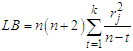 | (8) |
where  is the auto-correlation of lag
  for the estimated residuals
  . Given the monthly seasonality of tourist arrivals, we set
  . Large values of LB lead to the rejection of the hypothesis of no auto-correlation between the residuals.
3. Point and Interval Forecasts
To make the managerial decision discussed in Section 1 operational, there is the need to forecast tourist arrivals  at month
  . Let
. Let  be the conditional expectation of
  given the past arrivals
  , that is,
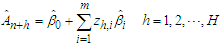 | (9) |
where  is a vector of known or prefixed values of explanatory variables at time
 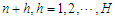 and
and  is a
is a  vector containing the ordinary least squares estimates of the parameters (intercept included). Let further
 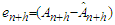 be the forecast error corresponding to
  . It follows from the Gauss-Markov theorem that
  is the forecast for which the mean squared error,
  , is as small as possible. Predictability is strictly entrenched with variability. The estimated variance of forecast errors is
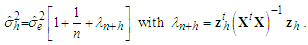 | (10) |
3.1. Assessing Point Forecast Accuracy
The main problem with assessing the reliability of forecasts is that the magnitude of forecast errors cannot be evaluated until the actual values have been observed. To simulate such a situation, we split tourist arrivals into two parts: the “training” period, which ignores a number of the most recent time points and the “validation” period, which comprises only the ignored time points. In this regard, arrivals observed in the period from January, 2018 to August, 2019 ( months) are set-aside to serve as a benchmark for forecasting purposes. Tourist arrivals from January, 2002 to December, 2017 act as training period. There are a number of indices that assess predictive accuracy. For our current purpose, we prefer an index that varies in a fixed interval and makes good use of the observed residuals. This is the relative absolute error of forecast (RAEF)
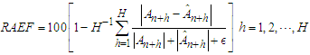 | (11) |
where  is a small positive number (e.g.
  ) which acts as a safeguard against division by zero. Coefficient (11) is independent on the scale of the data and, due to the triangle inequality, ranges from zero to 100. The maximum is achieved in the case of perfect forecasts:
  for each
  . The lower the
  is, the less accurate the model is. The minimum stands for situations of inadequate forecasting such as
  or
or  for all
  .
.
3.2. Simultaneous Prediction Intervals
In tourism marketing, planning, development and policy-making it is not only important to generate point forecasts for several steps ahead, but providing an assessment of the uncertainty associated with forecasts can be equally important. The problem is thus to integrate point forecasts with prediction intervals (PIs) which apply simultaneously to all possible future values of the predictors.A reasonable strategy can be as follows: Given the availability of  future values, we can construct two bands such that, under the condition of independent Gaussian distributed random residuals, the probability of consecutive future Arrivals
 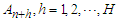 that lie simultaneously within their respective range is at least is
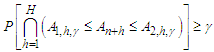 | (12) |
where 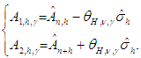 | (13) |
The multiplier  is the
  -th quantile of the of the maximum absolute value
  of the
  -variate Student
  probability density function with
  degrees of freedom. See [8]. In short,
  is the solution of
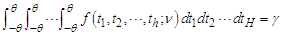 | (14) |
The critical values can be found solving iteratively  using the command
  of the
  package
  , which provides the multivariate
  probability. See [9].The most important characteristic of PIs is their actual coverage probability (PIAC). We measure PIAC by the proportion of true arrivals of the validation period enclosed in the bounds
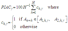 | (15) |
If  then future arrivals tend to be covered by the constructed bounds, but this may also imply that the estimates of the variances in the forecast errors are positively biased. A
  indicates under-dispersed forecast errors with overly narrow prediction intervals and unsatisfactory coverage behavior.All other things being equal, narrow PIs are desirable as they reduce the uncertainty associated with forecasts. However, high accuracy can be easily obtained by widening PIs. A complementary measure that quantifies the sharpness of PIs might be useful in this context. Here, we use the score function.
 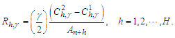 | (16) |
This expression reflects a penalty proportional to the narrowness of the intervals that encompass the true values at the nominal rate. The penalty increases as  decreases, to compensate for the tendency of prediction bands to be broader as the confidence level increases. Of course, the lower
  is, the more accurate PI will be. The average value of the score width across time points
 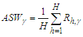 | (17) |
can provide general indications of PIs performance.
3.3. Application of the OLS Approach
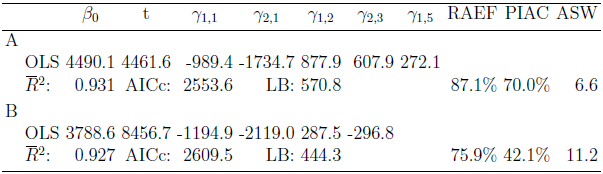
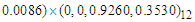
We have applied the OLS procedure outlined in the preceding section to monthly time series of Italian tourist arrivals (series A) and international tourist arrivals (series B). Table 1 shows the results obtained with ordinary least squares (OLS) applied to the data of the training period for the arrivals in the validation period. As it can be seen, nine predictors have been discarded for time series A and ten for time series B. The remaining predictors are significant at the 0.00001% level. The trend-cycle component in both cases is a simple linear function of the time, which implies that changes are constant, whereas the seasonal components are characterized by very few harmonics. Finally, the quality of fitting has generally been satisfactory because the adjusted R-square is always above 92%.Table 1. OLS estimation and forecasting
 |
| |
|
The major drawback of OLS is clearly found in the Ljung-Box statistic. The values reported for both time series are extremely high (with a  -values virtually zero), so indicating that auto-correlation in the OLS residuals has to be taken seriously into account.
4. A Reg-SARMA Model
Serially correlated residuals have several effects on regression analysis. OLS estimators remain unbiased but are not efficient in the sense that they no longer have minimum variance. Furthermore, forecast intervals and tests of significance commonly employed in OLS would no longer be strictly valid, even asymptotically (see, e.g. [10] [Ch. 8]). In general, the presence of auto-correlation reveals that there is additional information in the data that has not been exploited in the regression model. This is a fact of which we are fully aware since we have not included any sector-specific explanatory variables in the equation, which should explain tourist arrivals.To correct for auto-correlation, we assume that the residuals are generated by a multiplicative SARMA process 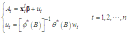 | (18) |
where  is a
is a  vector of the predictors remained in the regression model (intercept included) of the first stage and
  are independently and identically distributed Gaussian random variables with zero mean and variance
  . Notice that the first equation is just a linear regression, and the second equation just describes the residuals as a Box-Jenkins process. One reason for this specification is that the estimated parameters retain their natural interpretations.The symbol
  in (18) denotes the usual backward shift operator
  and
and  and
and  are polynomials in
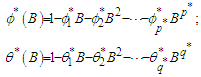 | (19) |
The polynomials in (19) are constrained so that the roots of  and
and  have magnitudes strictly greater than one, with no single root common to both polynomials, that is, only processes which are stationary and invertible are considered. Some of the
  and
and  could be set equal to zero. Process (18) do not include difference operators because the “burden of non-stationarity” is placed entirely on the orthogonal polynomials and harmonics used as predictors. Let
  be the estimated residuals from OLS regression where
  are the fitted monthly arrivals. We can express the OLS residuals as
 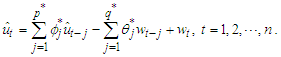 | (20) |
Equation (20) contains some indeterminacies: the residuals  and the errors
  are unknown and cannot be determined within the context of model (20). We regard residuals and errors that might be supposed to exist before the initiation of the active process as fixed constants and set to zero the errors
  because, after all, zero is their expected value. The residuals
  are set equal to the last OLS residuals in reverse time order. In this way, we avoid the detrimental impact that the zeros could have on the estimation results in the case of small or moderate length of the time series. Given the above conditions, the unknown parameters
  and
and  can be estimated by optimizing the log-likelihood function of the SARMA process. However, since we ignore the orders of autoregressive-moving average components, the estimation must be repeated for each reasonable value of
  and
and  . It is well known that any stationary and invertible
  process can be expressed as an infinite auto-regression
  and that the coefficients in
  may be virtually zero beyond some finite lag. Based on these premises, many authors (e.g. [11], [12],) suggested a pure auto-regressive process (up to a prefixed large lag) as a model for the regression residuals. In our experience, however, this opportunity not only implies a high number of parameters due to seasonality, but also does not wholly eliminate serial correlation.A controversial, but proved technique to find a good choice for
  and
and  is a trawling search through a grid of possible processes fine enough to produce meaningful results and the process with the lowest AICc value selected. Usually, brute-force methods are unmanageable for long time series because of the computational complexity. Notice that process (18) may be considered as special case of the standard ARMA
  by taking
  ,
,  . The integer
  is the seasonal period (
 for monthly time series). For example, if
  then the search involves estimating 144 different processes, which may seem cumbersome in terms of computational efforts at first. Actually, the obstacle is more apparent than real. Improvements in computer technology and reductions in hardware costs make the trawling search solution attractive for much more research and real-world applications than in the past. We have examined 144 different SARMA models and choose the stationary and invertible process
  with the minimum Ljung-Box statistic.Let
  and
and  . The fitted OLS residuals produced by the best SARMA process are
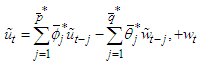 | (21) |
where  are the errors of the fitted SARMA process. The first stage of the Reg-SARMA approach terminates with a re-specification of the regression equation explaining tourist arrivals:
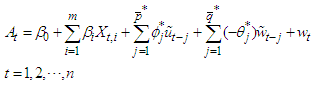 | (22) |
which contains  additional pseudo regressors. Predictors
  in the last sum on the right-hand side of (22) are, by construction, pairwise uncorrelated and do not contribute to the multi-collinearity of the new regression model. Even the estimated residuals
  do not appear to carry significant additional problems of multi-collinearity. The second stage of the Reg-SARMA approach consists of the OLS estimation of (22) to whom it can be plenty applied the classical linear regression theory because now the theoretical residuals are uncorrelated. The presence of lagged values of the response variable on the right hand side of the equation mean that the regression parameters can only be interpreted conditional on the value of previous values of the response variable.It must be pointed out that the Reg-SARMA approach outlined above is not the same as a regression model with SARMA errors, which is part of the R package forecast [13] or the same as the ARIMAX procedure as implemented in the package TSA. However, in our experience, these methods yield equivalent results.
4.1. Properties of Reg-SARMA Estimators
Let  be the
  matrix constructed by using the OLS residuals fitted by the best SARMA process, with
  being the maximum lag of the auto-regressive component. Each column of
  is a time series of
  at lags
  . Analogously, let
  be the
  matrix constructed by using the estimated errors of the best process with
  being the maximum lag of the moving average component. Each column of
  is a time series of
  at lags
  . The design matrix of the final model at the final stage is therefore given by
  . To assess the sample properties of the Reg-SARMA estimators the term
  requires making explicit assumptions. 1. The conditional expectation of
  given the predictors for all time periods, is zero:
  for each
  .2. No predictor is constant or a perfect linear combination of the others.3. The conditional variance
  is finite and constant for each
  .4. Conditional on the matrix of predictors
  , the residuals in two different periods are uncorrelated with each other
  for each
  .5. The
  are independently and identically distributed as Gaussian random variables with zero mean and finite variance
  .If conditions 1-4 are satisfied then the Reg-SARMA estimators are the best linear unbiased estimators conditional on
  . The variance of the estimators is given by
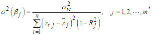 | (23) |
where  and
and  is the
  -squared from the regression of
  on the other predictors. An unbiased estimator of the variance of the
  is
is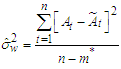 | (24) |
Condition 5 implies 3 and 4, but it is stronger because of the independence and Gaussianity assumptions. A direct consequence is that the least squares estimators have a Gaussian distribution, conditional on  , providing in this way, an inferential framework for the Reg-SARMA model.
4.2. Forecasts in Reg-SARMA Models
The Reg-SARMA (22) can produce predictions of the new arrivals 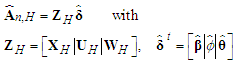 | (25) |
where  ,
,  is, as before, the time horizon of forecast and
  is a
is a  matrix of the
  predetermined values of the predictors for
  . The
. The  matrix
  is constructed by using the OLS residuals forecast by the best SARMA process and
  is the maximum lag of the auto-regressive component. Each column of
  includes forecast of
  at lags
  and
and  . Analogously, the
  matrix
  is matrix constructed by using the forecast errors of the best process and
  is the maximum lag of its moving average component. Each column of
  is a time series of
  at lags
  and
and  . The preceding discussion assumes that the future values
  are known without errors or can be forecast perfectly or almost perfectly, ex ante. If, on the contrary,
  or part of it must themself be forecast then formula (25) has to be modified to incorporate the uncertainty in forecasting
  . [14] [Section 4.6.4] points out that firm analytical results for the correct forecast variance for this case remain to be derived except for simple special situations. In the case of the Reg-SARMA model (22), explanatory variables
  are deterministic, but
  and
and  are not because these “pseudo” regressors contain random variation due to estimation errors. It follows that, the application of the prediction intervals in (12) to the Reg-SARMA model is based upon the strong and unrealistic assumption of making correct inference as if the serial correlation structure of regression residuals follow exactly or almost exactly the best SARMA process. It is clear that this assumption can be the subject of discussion. We claim, however, that in many circumstances this hypothesis can be as valid as making the assumption that the explanatory variables are non-random, or fixed in repeated samples.
4.3. Empirical Analysis
In the case of arrivals from Italy the SARMA process has been identified as the best description of OLS residuals in terms of Ljung-Box criterion with parameters
  . In the case of arrivals from all the other countries, the best process is
  with parameters
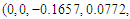
 . The R scripts for computing the Reg-SARMA estimates are available from the author on request. Table 2 shows the results obtained with the Reg-SARMA method applied to the data of the training period for the arrivals in the validation period. The Reg-SARMA approach offers several improvements over OLS. The auto-correlation is almost inexistent because the
  -value of the LB statistics is now larger that 999%. Also, the quality of the fitting is increased as proven by a lower AICc and a higher
  than those observed for OLS.
Table 2. OLS and Reg-SARMA estimation and forecasting
 |
| |
|
In both cases the amelioration is quite substantial. In addition, as can be readily seen from Figure 2, the coverage rate is now significantly higher compared to OLS. The cost of these enhancements is a larger width of the simultaneous forecast intervals, which, as it is well known determine broader brackets than marginal (and wrong) classical OLS intervals. Furthermore, the stability of the RAEF index across the two estimation methods, is a demonstration that the predictive accuracy does not deteriorate when Reg-SARMA method is used. Nonetheless, we must remark that, both OLS and Reg-SARMA methods, yield prediction intervals whose actual coverage rate resulted to be less than the nominal level (90%) (the latter are better than the former). We explain this result as due to a change in the evolutionary trajectory of arrivals to Italy, which in the last two year, has not been following the trends of previous years. This is an obvious consequence of the need of bracketing future values within the same scheme used for past observations. Thus a constraint is imposed on the forecasting tool: strong local fluctuations or outliers cannot appear in the set of future values even if we know that they are there; thus, some failures are inevitable.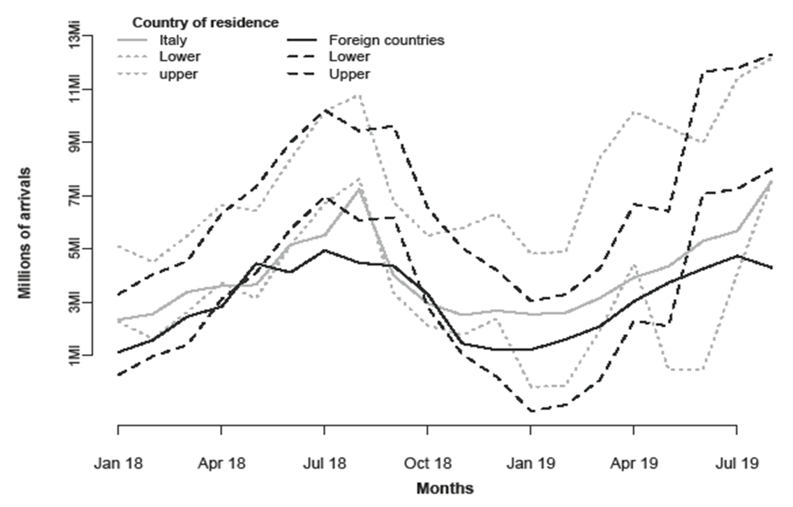 | Figure 2. Forecast of arrivals to Italy |
5. Concluding Remarks
When the hypothesis of independency in the residuals of a regression model may not be satisfied, bias and misinterpretation in the estimated parameters and computed statistics are very likely. In this paper, we have assumed that the regression residuals arise from a seasonal auto-regressive moving average stochastic model. In this way we have not only eliminated serial correlation from the regression residuals, but also constructed valid simultaneous prediction intervals to contain future monthly arrivals to Italy, according to the country of residence of guests.Some tentative conclusions can be drawn from this application, but their general validity can be substantiated only by further experience with the method. First of all, we have to point out the strong trade-off between auto-correlation and width of the simultaneous prediction intervals. Therefore, it cannot be excluded that the cure could be worse than the disease. We do not mean to discourage the regression with SARMA residuals, which may be the only realistic way forward in the absence of a renewed effort to introduce new (and practical) solutions to the inefficiency of ordinary least squares in case of serially dependent residuals. Accordingly, from a prudential point of view, it might be in one's self-interest to maintain a conservative attitude toward forecasting operations.On the other hand, we cannot be too severe on the new method, because it should not be forgotten that the behavior of the time series under investigation in the validation period is distinct from that in the training period. Nevertheless it is important to recognize that the Reg-SARMA approach even if eliminates auto-correlation, brings important costs of its own, and it does not eliminate problem with the variance of the predicted values.
References
| [1] | Sun, S., Wei, Y., Tsui, K., Wang, S. (2019). Forecasting tourist arrivals with machine learning and internet search index. Tourism Management, 70, 1-10. |
| [2] | Frechtling, D. C. (2001). Forecasting Tourism Demand: Methods and Strategies, Butterworth-Heinemann, Oxford. |
| [3] | Witt, S. F., Witt, C. A. (1995). Forecasting tourism demand: A review of empirical research. International Journal of Forecasting, 11, 447-475. |
| [4] | Istat (2019) http://dati.istat.it/?lang=en&SubSessionId=3ba6303c-bc4b-4fd2-b355-3df94526ae47. |
| [5] | Chateld, C. (2000). Time series forecasting. Chapman & Hall/CRC, Boca Raton. |
| [6] | Chan, K.-S., Ripley, B. (2018). TSA: Time Series Analysis. R package version 1.2. https://CRAN.R-project.org/package=TSA. |
| [7] | Ljung, G. M., Box, G. E. P. (1978). On a measure of lack of t in time series models. Biometrika, 65, 297-303. [Makoni & Chikobvu, 2018] Mak 2018 Makoni, T., Chikobvu, D. (2018). Modelling and Forecasting Zimbabwe, Äôs Tourist Arrivals Using Time Series Method: A Case Study of Victoria Falls Rainforest. Southern African Business Review, 22, 1-22. |
| [8] | Hahn, G. J. (1972). Simultaneous prediction intervals for a regression model. Technometrics 14, 203-214. |
| [9] | Genz, A., et al. (2019). Multivariate Normal and t Distributions. R package version1.0-11, https://CRAN.R-project.org/package=mvtnorm. |
| [10] | Chatterjee, S., Hadi, A. M. S.: Regression Analysis by Example (4h ed). John Wiley & Sons, New York (2006). |
| [11] | Pukkila, T., Koreisha, S., Kallinen, J. (1990). The identication of ARMA models. Biometrika, 77, 537-548. |
| [12] | Koreisha, S. G., Fang, Y. (2008). Using least squares to generate forecasts in regressions with serial correlation. Journal of Time Series Analysis, 29, 555-580. |
| [13] | Hyndman, R. J., Khandakar, Y. (2008). Automatic time series forecasting: the forecast package for R. Journal of Statistical Software, 26, 1-22. http://www.jstatsoft.org/article/view/v027i03. |
| [14] | Green, W. H.: Econometric Analysis (7th Edition): International edition. Pearson Education Limited (2012). |
| [15] | McLeod, A. I., Zhang, Y. (2008). Improved subset autoregression: with R Package. Journal of Statistical Software, 28, http://www.jstatsoft.org/v28/i02/. |

 Abstract
 Reference
 Full-Text PDF
 Full-text HTML