Md. Mynul Islam1, Mohiuddin Ibn Shafique2, Md. Abdur Rahman3, Mohammad Lutfor Rahman1
1Institute of Statistical Research and Training, University of Dhaka, Dhaka, Bangladesh
2United Nations Development Programme (UNDP), IDB Bhaban, Shar-E-Bangla Nagar, Agargaon, Dhaka, Bangladesh
3Bangladesh Meteorological Department, Agargaon, Dhaka, Bangladesh
Correspondence to: Md. Mynul Islam, Institute of Statistical Research and Training, University of Dhaka, Dhaka, Bangladesh.
| Email: |  |
Copyright © 2021 The Author(s). Published by Scientific & Academic Publishing.
This work is licensed under the Creative Commons Attribution International License (CC BY).
http://creativecommons.org/licenses/by/4.0/

Abstract
A time-series modeling tool SARIMA (4,0,4)(1,1,1) [12] model has been implemented to project the total number of monthly thunderstorm-days at 34 different meteorological stations in Bangladesh. Efforts have been made to determine, as accurate as possible, the future number of thunderstorm-days up to five years. Detailed modeling procedure and forecasting accuracy are demonstrated. Due to the recent unusual rise in the number of deaths from lightning in Bangladesh, this research will be useful for policymakers to take the necessary precautions.
Keywords:
Thunderstorm, Bangladesh, Time series modeling, SARIMA, Forecasting
Cite this paper: Md. Mynul Islam, Mohiuddin Ibn Shafique, Md. Abdur Rahman, Mohammad Lutfor Rahman, Forecasting Thunderstorms in Bangladesh: A Time Series Modeling Approach, International Journal of Statistics and Applications, Vol. 11 No. 1, 2021, pp. 1-7. doi: 10.5923/j.statistics.20211101.01.
1. Introduction
Lightning is one of the vital meteorological parameters considered around the world to monitor climate change [1]. Nearly 45000 lightning occurs every day [2]. Lightning is a large electrical discharge created from a thundercloud. It is the flashlight, we see, during that electrical discharge. Besides, thunder is the sound we get from lightning. Lightning and thunder create a thunderstorm. On the negative side of lightning, after tornadoes, flash floods, and hurricanes, it is considered as the leading cause of weather-related deaths [3]. It causes a considerable number of causalities (with 24,000 deaths per year) and damages of properties [4]. Because of the spatial organization of Bangladesh, with the Himalaya in the north and the Bay of Bengal in the south, this land is a vulnerable region of a natural disaster like storm, drought, flood, thunderstorms. Compared to high-income countries, Bangladesh, a densely populated country, faces a higher number of fatalities due to thunderstorms [5]. For instance, fatality from the lightning is calculated within the range from .2 to 1.7 deaths/1000000 population over the world. And in Bangladesh, the fatality rate is .9/1000000 which is higher than high-income countries [6]. Since Bangladesh had been witnessing an increasing trend in the number of deaths by lightning, the government of Bangladesh declared it a natural disaster in 2016 [7]. Nevertheless, only a handful number of researches can be found on lightning and thunderstorm in this region. Tyagi et al. [8] have documented the history of pre-monsoon thunderstorms over the Indian region, particularly about nor’easters over eastern and Northeast India. But no study has so far been made on the frequency of thunderstorms and thunderstorm days in Bangladesh except [9]. While the ARIMA model can support to analyze a trend, SARIMA model can do both trend and seasonality. For seasonal time series, Box and Jenkins presented this successful type of ARIMA model by including the seasonal part to develop the model [10]. In this paper, to analyze the frequency of thunderstorm days, seasonal autoregressive integrated moving average (SARIMA) model has been implemented. Furthermore, to verify the assumptions, randomness, independence, and normality of the residuals have been carried out.
2. Methodology
A time series is a sequence of observations of a random variable generated through a stochastic process measured at equally spaced time intervals. The key purpose of time series modelling is to carefully characterize the process through the past observations of the time series by developing an appropriate model which explain the inherent structure of the series. Thus, this model can facilitate to forecast the process. There are several approaches to modelling series with seasonal pattern. Among these are exponential smoothing [11]), seasonal ARIMA models [10], state- space models [12] and the innovations State Space Models [13]. ARIMA model is widely used to analyze the trend of the series and forecast future values. Rahman et al. [19] utilized the ARIMA model for modeling inflation over time in Bangladesh. ARIMA models for time series data have the potentiality to represent stationary as well as non-stationary time series and to generate correct forecasts based on available historical data of single or multiple variable. Since it does not allow any systematic pattern in the previous data of series that are to be forecasted, this model is very distinct from other models used for forecasting. This model was developed by [10] and [14].This model is composed of three components. An autoregressive integrated moving average (ARIMA) models is denoted as ARIMA (p, d, q). ARIMA model can explain temporal dependence in various ways. Firstly, the series is d-differenced to make it stationary. When d = 0, the observations are considered stationary and modelled directly, and when d  1, the differences between consecutive observations are modelled. Secondly, the time dependence of the stationary process Xt is modelled by including autoregressive models of order p. The equation for order p is:
 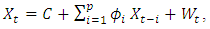 | (1) |
where, C is a constant,  is the autoregressive parameter,
  is the observed value at time t and,
  represents random error. The third component is moving-average term of order q. It considers the observation of previous random errors. The equation for order q is:
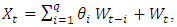 | (2) |
where, C is a constant,  is the model parameter,
  is the error term. Finally, by combining these three components, we obtain the ARIMA model. Thus, the general form of the ARIMA models can be expressed as:
  | (3) |
Generally, ARIMA models use the back-shift operator B which is defined as  where k is the index representing how many times back-shift operator B is applied to time series
  characterised by time interval t, and N is the total number of time intervals. Using the following notations
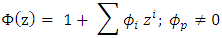
 the Eq. (3) can be written as
  The seasonal ARIMA (p, d, q) (P, D, Q)[m] process noted also as SARIMA (p, d, q) (P, D, Q)[m] is given by:
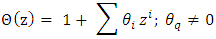
 where m is the seasonal period, φ(z) and Θ(z) are polynomials of orders P and Q, respectively, each containing no roots inside the unit circle. If c
  0, there is an implied polynomial of order d + D in the forecast function [15,16]. To determine an appropriate model for a given time series data, it is necessary to figure out the Autocorrelation Function (ACF) and Partial Autocorrelation Function (PACF) analysis, which reflects how the observations in a time series are interrelated. The plot of ACF helps to determine the order of Moving Average terms, and the plot of PACF helps to find Autoregressive terms.The main task in SARIMA forecasting is selecting an appropriate model order; that is, the values p, q, P, Q, D, d. If d and D are known, we can select the orders p, q, P and Q via one of the forecast measure error: the mean absolute error (MAE), the root mean squared error (RMSE) and the mean absolute scaled error (MASE). MAE and RMSE are defined by the formulas:
 respectively, where n is the number of periods of time and
  is the forecast error between the true value
  and the forecasted value
  . The MAE is the average value over the sample of the absolute values of the differences between the forecast and the corresponding observation. Moreover, the RMSE is the square root of the average squared values of the differences between forecast and the corresponding observation. These errors have the same units of measurement and depend on the units in which the data are measured. The MASE was proposed by [17] for comparing forecast accuracies. The MASE is given by the formula:
  where Q is a scaling statistic, computed on the training data. For a non-seasonal time series, a useful way to define scaling statistics is to apply the mean absolute difference between the consecutive observations:
  that is, Q is the MAE for naive forecasts, computed on the training data. The MASE is less than one if it arises from a better forecast than the average naive forecast computed on the training data. Conversely, it is greater than one if the forecast is worse than the average naive forecast computed on the training data. For a seasonal time series, a scaling statistic can be defined using the seasonal naive forecasts:
  where the seasonal naive method accounts for seasonality by setting each prediction to be equal to the last observed value of the same season. The MASE is independent of the scale of the data, so it can be used to compare forecasts for data sets with different scales. When comparing forecasting methods, the method with the lowest MASE is the preferred one. Therefore, the approach of Box-Jenkins methodology in order to build ARIMA models is based on the following steps: (1) Model Identification, (2) Parameter Estimation and Selection, (3) Diagnostic Checking (or Model Validation); and (4) Model’s use.
3. Data
The study data were collected and provided by Bangladesh Meteorological Department, Climate Division, Dhaka. The data contain information about monthly number of thunderstorm-days for 34 different meteorological stations of Bangladesh from 1980 to 2018. The locations of the stations are represented in Figure 1. This study is design to forecast total number of thunderstorm-days in Bangladesh. Monthly total number of thunderstorm-days in Bangladesh is calculated by taking sum of monthly thunderstorm- days over 34 different stations. 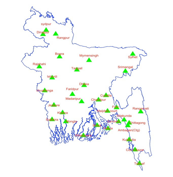 | Figure 1. Locations of the meteorological stations in Bangladesh |
4. Results and Discussions
The first step of time series analysis is to plot the series against time which is called the time plot. The time plot of total number of thunderstorm-days for the period 1980 to 2018 is shown in Figure 2. In-spite of being there no visible trend of total number of thunderstorm-days in the figure, seasonality is visible there (Figure 2 and Figure 3). The maximum number of thunderstorm-days occurs in May. The number of thunderstorm-days increases from January to May which remains similar to September, then it again decreases. Fewer numbers of thunderstorms-days occur in November, December, and January. 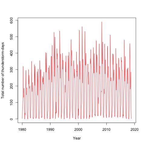 | Figure 2. Graphically visualizing monthly total number of thunderstorm-days in Bangladesh from the year 1980 to 2018 |
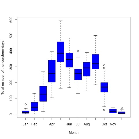 | Figure 3. Month wise box plot for total number of thunderstorm-days in Bangladesh |
For the additive decomposition of the series in Figure 4, it seems that in the series, there is no linear-trend- which is also confirmed by applying the sieve-bootstrap version of the t-test by adapting the approach of Noguchi, Gel, and Duguay [21]. This t-test fails to reject the null hypothesis of no-trend with a t-value of 1.994 and a p-value of 0.875.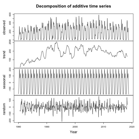 | Figure 4. Decomposition of the series |
Original series in Figure 2, Figure 3 and additive decomposition of the series in Figure 4 showed no stationary of data due to the presence of seasonality. Likewise, the graph of the ACF’s of the original series in Figure 5 showed not stationary data because the autocorrelation after lag time 1 quite significantly from zero that decreases very slowly. 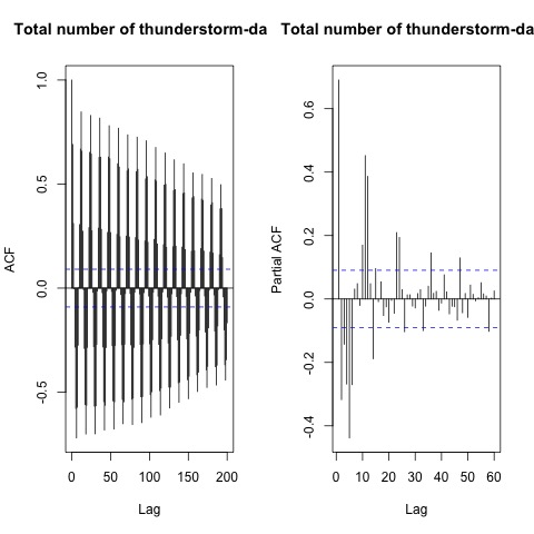 | Figure 5. ACF and PACF of the series |
If the mean and the variance of the series are independent of time, but rather are constants and their covariance at different lags does not depend on time, the series is said to be a stationary series. This series seems to non-stationary as its mean is not constant over the time. Moreover, statistical testing can be used to verify the stationarity of considered series. To do this, there are two different approaches: stationarity tests such as the Kwiatkowski-Phillips-Schmidt-Shin (KPSS) test that consider the null hypothesis as the series is stationary, and unit root tests, such as the Dickey-Fuller test and its augmented version, the augmented Dickey-Fuller test (ADF) for which the null hypothesis is thought as the series is not stationary. ADF test suggest the non-stationarity of our series with p-value 0.2391 higher than 0.05, which was also confirmed by the KPSS test. Thus, the series is not required the regular trend differencing. To make sure whether seasonal trend difference, D, is required, a seasonal unit root test (the HEGY test [20]) has been implemented. HEGY test suggests that there is a unit root with a statistic value -2.3033 and p-value 0.3866. Therefore, the series required the seasonal trend differencing, so in all SARIMA models, we assumed d = 0 and D = 1. Figure 6 that represent time plot of the first seasonal difference of the series shows stationary on the value of the data center because the graphics look along the horizontal axis of time. ACF Graph towards zero after one lag. Autocorrelation values after a lag 4 does not differ significantly from zero or is within the limits of an autocorrelation values so that shows the stationary data. This shows a pattern for time series modeling once at deference’s. 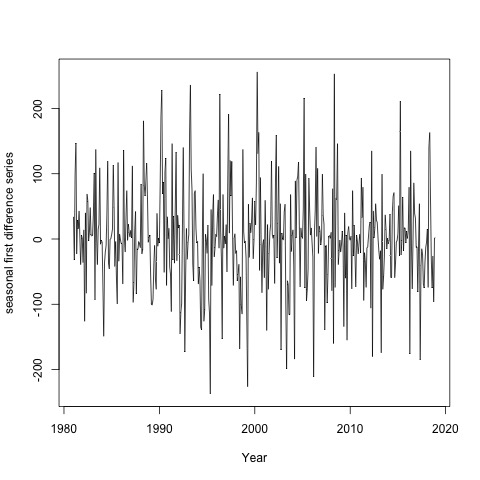 | Figure 6. Time plot of the seasonal first difference series |
Additionally, the ACF plots shown in Figure 7 depict a sine wave and show spikes in the seasonal lags 12. This effect significantly supports the evidence of seasonality in the data sets.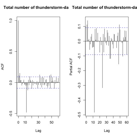 | Figure 7. ACF and PACF of the stationary series |
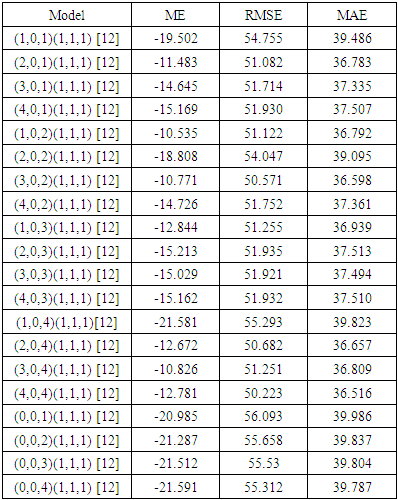
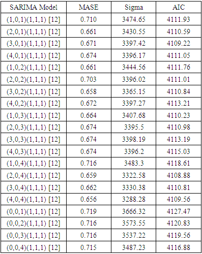
Identification of the model while the Figure 7 shows the values of the autocorrelation are insignificant after lag 2. This indicates the existence of a pattern of MA (Moving Average) takes two, MA (2) that is not seasonal. The seasonal pattern is still visible on the autocorrelation values data deference’s so strengthen the presence process MA (1) seasonal. There are two value of a very significant partial autocorrelation at lag 1 and 2 so assumed the existence of a pattern of AR (Autoregressive) takes two or AR (2) is not seasonal. The seasonal pattern is still visible on the partial autocorrelation values data deference’s so strengthen the presence process AR (2) seasonal. Based on this, the candidate model is ARIMA (2, 0, 2), (2, 1, 1), D = 1, and s = 12. In this study, data were from 468 months in the period between January, 1980 and December, 2018 and the data set was partitioned into a training set and a test set. All the observations from January, 1980 to December, 2011 were taken into consideration as the training set and were applied so as to fit the created statistical models for the Total number of thunderstorm-days. The data from January, 2012 to December 2018 were designated as the test set and were used to assess the predictability accuracy of the fit. This approach gives the ability to compare the effectiveness of different methods of prediction. by minimizing the forecast measure errors RMSE, MAE, MASE and AIC. In this study, 20 models with seasonal parameter (P = 2, D = 1, Q = 1) and 20 models with seasonal parameter (P = 1, D = 1, Q = 1) is considered. It is seen that models with seasonal parameter (P = 1, D = 1, Q = 1) has minimum value for the model accuracy parameters. Thus, we chose the best parameters of SARIMA models among the considered 20 models with seasonal parameter (P = 1, D = 1, Q = 1). SARIMA (4,0,4) (1,1,1) [12] and SARIMA (2,0,4) (1,1,1) [12] model was selected as the most appropriate from all 20 tested SARIMA models for thunder (Table 1 and 2). Table 1. Estimated values of the model accuracy parameters
 |
| |
|
Table 2. Estimated values of the model accuracy parameters
 |
| |
|
According the model accuracy parameters value (Table 1 and 2) and Figure 8 it can be inferred that selected SARIMA models are reasonable to forecast total number of thunderstorm-days in Bangladesh. 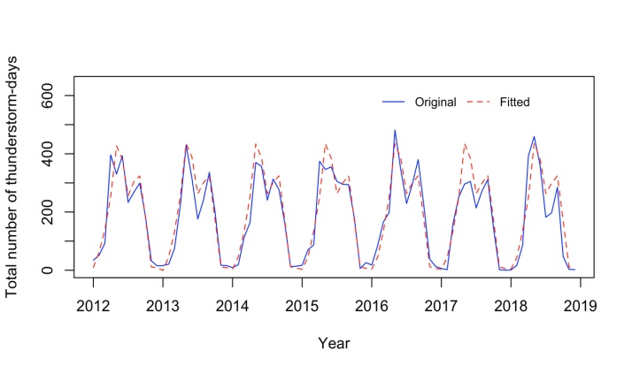 | Figure 8. Fitted value vs original series (test data) from the selected SARIMA model |
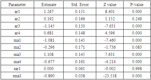
Estimation and testing significance of the parameters of the appropriate model has been accomplished in this section. From the previous analysis we have found that SARIMA(4,0,4)(1,1,1) [12] would be the best model. Parameters of the SARIMA model obtained by fitting the model are shown in TABLE 3 with corresponding significance value. The forecasted value of the monthly total number of thunderstorm-days in Bangladesh with 95% confidence limits have been displayed graphically in Figure 9.Table 3. Estimated parameters of the SARIMA model
 |
| |
|
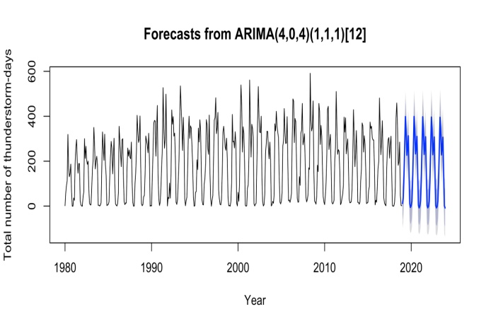 | Figure 9. Graphical display of the forecasted values of the monthly total number of thunderstorm-days in Bangladesh |
It is necessary to do diagnostic checking for the model adequacy although the selected model might appear to be the best model. This is done by studying the residuals. Randomness and independence of residuals are two important assumptions in modeling. Without these two properties good results from the model cannot be expected. Graph of residuals shows whether residuals are random or not. If there is no pattern in the residuals, we might assume that the residuals are randomly distributed. The ACF of residuals shows whether residuals are independent or not. If there is no point outside the line, we can conclude that residuals are independent. Large p-values of Ljung Box test indicate that residuals are white noise. From the first plot in Figure 10, it is found that residuals are scattered both sides of zero line without making any pattern. Therefore, it is believed that residuals are randomly distributed. From the second graph in Figure 6, we notice that none of the points are outside the significance line which proves the independence of residuals. In Ljung Box test, Chi-square value is 11.77 with 20 degrees of freedom and test p-value is 0.935 that indicate that residuals do not follow any specific pattern at 5% level of significance. Therefore, the null hypothesis of independence cannot be rejected and we conclude that residuals are independent in nature. Normality of residuals of a model is also another important assumption. If normality assumption of residuals of a model is violated, the model will entail misleading inferences. Histogram of the residuals in Figure 10 suggest us that the residuals are might be generated through a normal process. The normality assumption of the residuals is also checked through the Jarque Bera test [22]. For the presence of outliers in the residuals, the Jarque Bera test rejects the null hypothesis of normality of the residuals with a p-value < 0.001. After eliminating the outliers from the residuals, the Jarque Bera test shows the residuals are normally distributed with a p-value of 0.1196.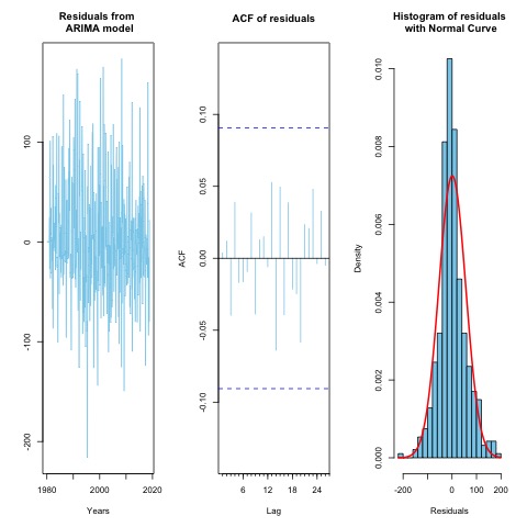 | Figure 10. Residual diagnostic plot |
5. Conclusions
Thunder occurs during a lightning storm as a result of acoustical effect of high temperature and pressure. Thus, the sound caused by lighting during lighting storm is called thunder. If the highest pressure in a storm happens a little distance away from the origin of the lightning strike, it causes a rumbling noise. The shock wave in thunder is sufficient to cause property damage [18] and injury, such as internal contusion, to individuals nearby.Thunder can rupture the eardrums of people nearby, leading to permanently impaired hearing [18]. Even if not, it can lead to temporary deafness. 1990-1999: 30 deaths and 22 injuries per year; 2000-2009: 106 deaths and 72 injuries per year, and 2010-2017: 260 deaths and 211 injuries per year occurred in Bangladesh [6]. Considering the massive death toll due to lightning, in 2016, the Government of Bangladesh has declared it as a natural disaster [7]. So, it is evident that the thunder is a public health, social and economic issue. A historical data of 39 years of thunderstorm-days has been visualized using time series modeling tools. Based on the criteria of minimizing MAE, RMSE, MAE, MASE, and AIC, SARIMA (4,0,4) (1,1,1) [12] model has been selected as the best model to forecast the total number of thunderstorm-days occurred in Bangladesh. Forecasting results using SARIMA model might be very useful to have an insight about the monthly occurrence of thunderstorm-days in Bangladesh and thus it might help the policymakers to take necessary effective measures to reduce the deaths, disabilities, damage as well as related burden in Bangladesh.
Declarations
Ethics approval and consent to participate A secondary dataset was used to conduct the current study, therefore no ethical approval was needed. Consent for publication All authors have given consent to publish the paper. Availability of data and material The dataset analyzed in this study is not publicly available but would be provided upon request. Competing interests There are no financial and non-financial competing interests for this study. Funding There was no funding for this study.
References
| [1] | Calvin, W. H. (2008). Global fever: how to treat climate change, University of Chicago Press. |
| [2] | Tessendorf, S. A., Rutledge, S. A., and Wiens, K. C. (2007). Radar and lightning observations of normal and inverted polarity multicellular storms from steps. Monthly Weather Review, vol. 135(11), pp. 3682–3706. |
| [3] | Biswas, A., Dalal, K., Hossain, J., Baset, K. U., Rahman, F., and Mashreky, S. R. (2016). Lightning injury is a disaster in Bangladesh?-exploring its magnitude and public health needs. F1000Research, vol. 5. |
| [4] | Jensen, J. D. and Vincent, A. L. (2019). Lightning injuries. In StatPearls [Internet]. StatPearls Publishing. |
| [5] | Chakravorti B., Kundar, M., Moloy, J. D., Islam, J., and Faruque, S. (2015). Earthquake forecasting in Bangladesh and its surrounding regions. European Scientific Journal, vol. 11(18). |
| [6] | Rahman, M. M. S., Hossain, M. S., and Jahan, M. (2019). Thunderstorms and lightning in Bangladesh. Bangladesh Medical Research Council Bulletin, vol. 45(1), pp.1–2. |
| [7] | Voa (2016). Bangladesh declares lightning strikes a disaster as deaths surge. https://www.voanews.com/east-asia/bangladesh-declares-lightning-strikes-disaster-deaths-surge. |
| [8] | Tyagi, B., Krishna, V. N., and Satyanarayana, A. (2011). Study of thermodynamic indices in forecasting pre-monsoon thunderstorms over kolkata during storm pilot phase 2006–2008. Natural hazards, vol. 56(3), pp. 681–698, 2011. |
| [9] | Karmakar, S. and Alam, M. (2005). On the probabilistic extremes of thunderstorm frequency over bangladesh during the pre-monsoon season. Journal of Hydrology and Meteorology, pp. 41–47. |
| [10] | Box, G. E. and Jenkins, G. M. (1970). Time series analysis: Forecasting and control holden-day. San Francisco, pp. 498. |
| [11] | Winters, P. R. (1960). Forecasting sales by exponentially weighted moving averages. Management science, vol. 6(3), pp. 324–342. |
| [12] | Harvey, A. C. (1990). Forecasting, structural time series models and the Kalman filter. Cambridge university press. |
| [13] | Hyndman, R., Koehler, A. B., Ord, J. K., and Snyder, R. D. (2008). Forecasting with exponential smoothing: the state space approach. Springer Science & Business Media. |
| [14] | Box, G. E., and Tiao, G. C. (1975). Intervention analysis with applications to economic and environmental problems. Journal of the American Statistical association, vol. 70(349), pp. 70–79. |
| [15] | Madsen, H. (2007). Time series analysis. Chapman and Hall/CRC. |
| [16] | Brockwell, P. J., Davis, R.A., and Fienberg, S. E. (1991). Time series: theory
and methods. Springer Science & Business Media. |
| [17] | Hyndman, R. J. and Koehler, A. B. (2006). Another look at measures of forecast accuracy. International journal of forecasting, vol. 22(4), pp. 679–688. |
| [18] | Vavrek, R. J. (2020). The science of thunder. http://lightningsafety.com/nlsi_info/thunder2.html. |
| [19] | Rahman, M. L., Islam, M. and Roy, M., (2020). Modeling inflation in Bangladesh. Open journal of Statistics, vol. 10(6) pp. 998-1009, 2020. |
| [20] | Hyllebeerg,, S., Engle R., Granger C. W. J. and Yoo. B. S. (1990). Seasonal integration and cointegration. Journal of Econometrics, Elsevier, vol. 44(1), pp. 215-238. |
| [21] | Noguchi, K., Gel, Y. R., and Duguay, C. R. (2011). Bootstrap-Based Tests for Trends in Hydrological Time Series, with Application to Ice Phenology Data, Journal of Hydrology, vol. 410 (3-4), pp. 150-61. |
| [22] | Jarque, C. M., and Bera, A. K, (1980). Efficient test for normality, homoscedasticity and serial independence of residuals. Economic Letters, vol. 6(3), pp. 255-259. |

 Abstract
 Reference
 Full-Text PDF
 Full-text HTML