-
Paper Information
- Paper Submission
-
Journal Information
- About This Journal
- Editorial Board
- Current Issue
- Archive
- Author Guidelines
- Contact Us
International Journal of Statistics and Applications
p-ISSN: 2168-5193 e-ISSN: 2168-5215
2020; 10(6): 141-149
doi:10.5923/j.statistics.20201006.01
Received: Oct. 17, 2020; Accepted: Nov. 2, 2020; Published: Dec. 15, 2020

Estimation of Hill Growth Model Parameters by Linearization
 Abstract
 Reference
 Full-Text PDF
 Full-text HTML
Wonu Nduka1, Biu Emmanuel Oyinebifun2
1Ignatius Ajuru University of Education, Rivers State, Nigeria
2University of Port Harcourt, Choba, Rivers, Nigeria
Correspondence to: Wonu Nduka, Ignatius Ajuru University of Education, Rivers State, Nigeria.
| Email: |  |
Copyright © 2020 The Author(s). Published by Scientific & Academic Publishing.
This work is licensed under the Creative Commons Attribution International License (CC BY).
http://creativecommons.org/licenses/by/4.0/

This study is focused on the estimation of the Hill growth model parameters which is a non-linear model. In estimating these parameters, secondary data (amount of transmitted voltage against the time of different values) was used for illustration. Firstly, logarithm transformation was applied to Hill growth model to make it linear. Then, an iteration was used to run the linear regression model using Microsoft Excel Solver and Ordinary Least Square (OLS) estimates. The iterations were run using upper asymptote (or the initial parameter at t = 0) and the growth range parameter starting from (-0.2, -0.1, 0, 0.1, …) and (-0.75, -0.50, -0.25, 0, …) respectively. The iteration was run until the R-square convergence at 86.5%; indicating the estimated parameters are appropriate for the fitted model. The result was confirmed by two model criteria: Bayesian information criterion (BIC) and Akaike information criterion (AIC) used. Hence, the identified Hill growth (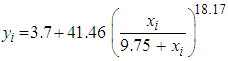 ) is adequate and can be used for forecasting of the amount of transmitted voltage against time.
Keywords: Hill Growth Model, Linearization, Model Selection Criterion, Linear Regression Model
Cite this paper: Wonu Nduka, Biu Emmanuel Oyinebifun, Estimation of Hill Growth Model Parameters by Linearization, International Journal of Statistics and Applications, Vol. 10 No. 6, 2020, pp. 141-149. doi: 10.5923/j.statistics.20201006.01.
Article Outline
1. Introduction
- Regression is a statistical model that can be used to explain the relationship between exogenous and endogenous variables (Ijomah et al., 2018). Hill model is a non-linear regression model with the four parameters
 and
and  A technique of finding a non-linear relationship between the dependent variable and a set of (or several) independent variable(s) called Non-linear regression analysis. In this way, non-linear regression is a function which models observational data by a non-linear combination of the model parameters and depends on one or more independent variables. As a result, many situations require non-linear function just like the simple and multiple linear regression functions that seem adequate for modelling a wide variety of relationships between the response variable and independent variables (Seber & Wild, 2003; Roush and Branton, 2005; Ijomah et al., 2018). In particularly, non-linear regression functions have served and will continue to serve as useful models for describing various physical and biological systems e.g. Hill growth model (or Hill model). Hill model is an S-shaped curve, often referred to as sigmoidal growth model (sigmoidal curve) which has many applications in agriculture, engineering field, signal detection theory also applicable in biochemistry, forestry (height distribution) and most importantly it is used in prediction. Numerous useful families of non-linear regression functions exist such as Richards, Logistics, Weibull, Gomperts, S. Shapes curves etc. These models are referred to as Sigmoidal Growth Models and are all useful in growth analysis. This study only considers Hill Model in growth analysis and its applications.The data used in this study is an experiment used to determine the amount of transmitted voltage against time collected from Department of Electrical/Electronic Engineering, University of Port-Harcourt. In some cases, it is possible to transform a non-linear regression function to a linear regression function using some appropriate transformations of the exogenous variable Yi, the parameters
  and
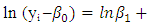
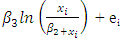
and  the endogenous variable Xi or any combination of these. If the assumptions for simple or multiple linear regression are satisfied in the transformed variables, then the result can be applied to the transformed problem. By the use of the transformed results, the original problem can obtain its results.The Hill model of growth with four parameters is expressed as
 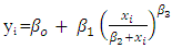 | (1.1) |
 are the parameters
 = represents upper asymptote when the time approaches positive infinite (or the initial parameter at time equal to zero; t = 0)
 = represents the shape parameter related to the initial time
 = represents growth range
  = represents the growth rate (or shape parameter) xi = represents time (Rudolf et al., 2012)Over the years, forecasting a non-linear model has been a major problem. On the course of solving this problem, many statistical models have been formed and transformed; the major tool for solving the problem is regression analysis (simple, multiple, linear or non-linear) for more accurate results, non-linear regression (growth models) has been developed for prediction, which includes: Hill (case study), Gomperts, Richards, Logistic, Weibull, Brody, Robertson etc.The custom statistical techniques in estimating nonlinear models require initial values to begin the optimization. The non-linear model expression must be written, the parameter names declared an initial parameter value specified. In most cases, the quality of the final solution depends upon the position of this initial value or starting value; after the iteration approach end. The problem of the initial parameter is solved (or reduced) by transformation to linear and OLS estimation before the iteration approach begins. This paper aims to estimate the Hill growth model coefficients/parameters using the equation of a line (simple linear regression). The objectives are as follows: (1) to derive the Hill Model to an equation of a line using transformation techniques (Logarithm) and its properties. (2) to choose the two initial values for the upper asymptote parameter
  and growth range parameter
  increasing by 0.1 and 0.25 rate respectively (3) to identify a suitable Hill Model and its parameters, using OLS estimation. There is a need to provide an alternative method of choosing the initial values and fitting the Hill growth model. This will provide an alternative way of a solution to this model and enable it to produce the desired level of forecasting. This paper only considers Hill model as a growth model neglecting other growth models such as Richards, Gompertz, Weibull, Brody, Robertson, Bertalanffy etc (Dagogo et al., 2018). Hence, an alternative way of solving Hill Model is explored in this study, where an iterative process, choosing initial values and OLS estimation is used in building the nonlinear model considered.
2. Review Works on Hill Growth Model
- The Hill model was first introduced by Archobald Vivian Hill who published the model first in its currently known form on 22th January 1910. This equation possesses three of the most important features of scientific models that is information, understanding and memorizing knowledge; it can be used to find an acceptable solution to practical problems, which we shall see in this review, and it can serve as a starting point for the development of a particular model and more detailed models. The Hill model is the first milestone in quantitative pharmacology research, being the first formula that reacts a reversible association (as an effect) to the variable concentration of one of two associating substances, as long as the other substance is present in a constant and relatively low concentration. Thereby, the Hill growth model was the first exact quantitative model in pharmacology that react to changes (or receptor model). The Hill equation (model) and its properties show that it is a good case study for understanding the development of quantitative models in life sciences.Carla et al., (2018), applied the Hills growth model to the treatment regimens that is the anti-microbial Pharmacokinetics (PK) and the antimicrobial Pharmacodynamic (PD) against the pathogen causing the disease. Their study aimed to use a model to analyze the relationship between the antimicrobial drug concentration and the pathogen populace. Their experiment captured the relationship between the antimicrobial drug concentration and its effect on the growth rate of the exposed pathogen population (Wen et al., 2018).Schmitt et al., (2013) researched on, muscle biomechanics, a vital and broad field. Given the research, it was known that in biology microscopic muscle models can predict muscle characteristics and functioning of biological muscles quite well; unfortunately, they require a large number of parameters like the Hill model. Zoran (2011) studied the relationship between the Hill function (model) and the more complicated Adair-Klotz model. He carried out an experiment using the dose-response curve, the result of the experiment showed that the curve (dose-response) obtained from Hill model agrees well with the dose-response curve obtained from Adair-Klotz Model describe strongly co-operative binding. Hence, the alternative technique suggested in the paper will help to construct a Hill model that its results indicate an improved analysis of growth performance, efficiency and the prediction of future or past growth rate.
3. Materials and Methods
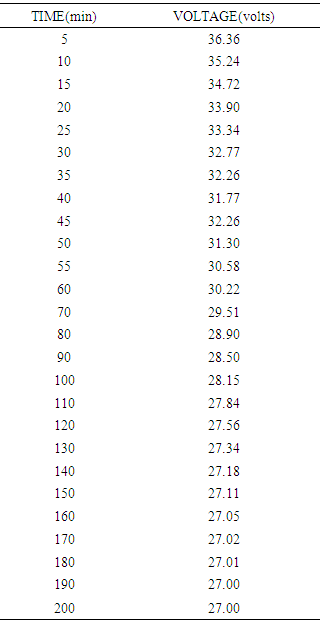
- - Materials A data set was considered in this project for the illustration of the fitted growth model. The data used in this study is an experiment used to determine the amount of transmitted voltage against time collected from the Department of Electrical/Electronic Engineering, University of Port-Harcourt (Appendix). The Microsoft Excel solver is used in the analysis of this study, however, there are others possibility for solving this kind of analysis such as Wolfram Mathematical, MATLAB, Minitab, Gretl statistical software’s etc. In the software’s, this problem (for all four parameters at once) can be fitted with a simple build-in command nonlinear model-fitting algorithm. - MethodsThe method of nonlinear least square estimation was applied by taking the derivatives concerning the parameters
 with additive and multiplicative error terms. A nonlinear regression model is similar to linear regression model both seek to graphically track a particular response from a set of predictor variables. Non-linear models such as Hill growth model in this work are developed because the function is created a series of approximations (iterations) that may stem from trial and error. Many researchers and statisticians use several established methods such as the Gauss-Newton method and the Levebberg-Marquardt method. This research work used the modified version of the Ordinary Least Square method that is1) Input the arbitrary value for
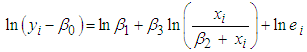
  as the initial guess values for the iteration process.2) Input the data and initial guess values on the Excel solver; then run the iteration to obtain the results. - Model SpecificationThe Hill Growth Model with Multiplicative error term (Rudolf et al., 2012), then Equation (1.1) can be expressed as
 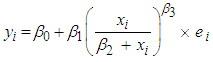 | (3.1) |
 are the error terms. Re-write Equation (3.1) as
 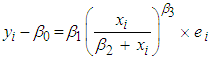 | (3.2) |
 | (3.3) |
 is the residual sum of squares of the model, where the number of parameters has been reduced from four to two parameters.Note:
 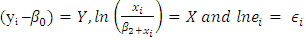 By applying the non-linear least square method, using step 1 and 2 above algorithms andLet
 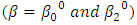 be the initial parameters as follow;
 and
and  = (-0.75, -0.50, -0.25, 0, …); where
  is increase by 0.1 and
  = is increased by 0.25.Note: One mathematical property of the Hill growth model is as follow;Asymptotes, if for
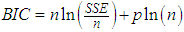
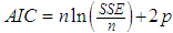
 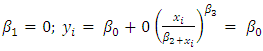 - Model Selection Criteria (1) R-Square (R2):The R-Square statistic measures the success of the regression in predicting the values of the dependent variable (Nduka & Ogoke, 2016). It assumes that every independent variable in the model help to explain variation in the dependent (y) and thus gives the percentage of explained variation if all independents in the model affect the dependent variable (y). The R2 statistic is defined as
 | (3.5) |
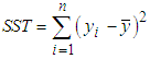 is the total sum of squares
 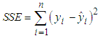 is the regression sum of squares
  and
and  are the original and modelled data values.(2) Adjusted R-Square (R2adj): In the least-squares regression, increasing the number of regressors in the model leads to an increase in R-Square. Hence R-Square alone cannot be employed as a meaningful comparison of the model. The adjusted R-Square (R2adj) tells us the percentage of variation explained by only those independent variables that do not belong to the model (Nduka & Ogoke, 2016).The adjusted R-square is defined as
 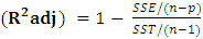 | (3.6) |
 | (3.7) |
 | (3.8) |

4. Analysis and Results
- The data in Appendix was used to build a suitable Hill growth model and its parameter estimates. Firstly, figure 4.1 scatter plot of the amount of transmitted voltage against time with a non-linear model called exponential model with its R2 value of 86.7%. This plot showed a slightly S-shaped curve and non-linear relationship between the amounts of transmitted voltage against time. Hence, a suitable Hill growth model can be identified.
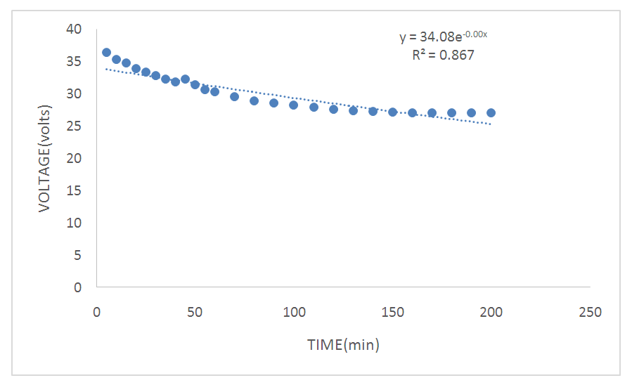 | Figure 4.1. Scatter plot of the amount of transmitted voltage against time |
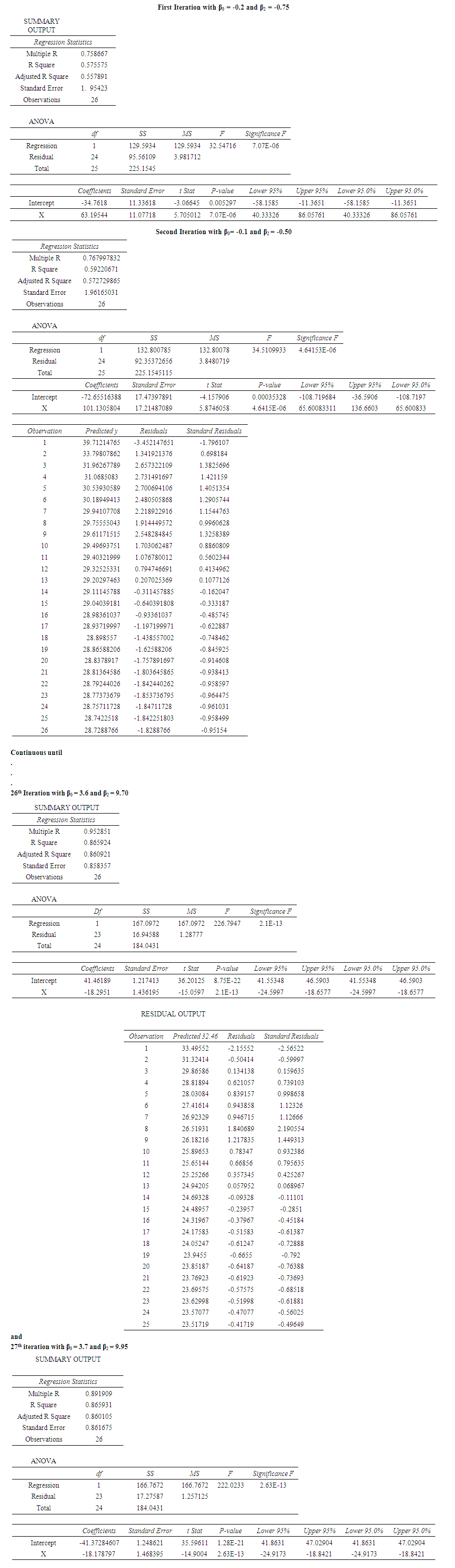
 as the initial guess values for the iteration process to start. Step 2: Then, input the data sets and the initial guess values on the Excel solver; then run the iteration to obtain the results OLS. Step 3: Continue the process (iterations) by increasing and decreasing arbitrary value for
  until the model selection criterion convergence; therefore stop the process.Table 4.1 below shows the values of the intercept and other parameters estimates with R2, Mean Square Error, AIC and BIC for various iterations. When
  increase by 0.1 and
  increase by 0.25.
|
 increase by 0.1);
  increase by 0.25)
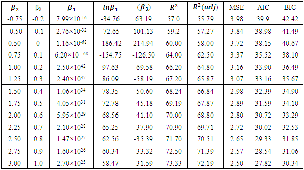
 from 0.1 to 0.3 and increase
  from 0.25 to 0.75 in Table 4.2.Similarity, Table 4.2 below shows the values of the intercept and other parameters estimates with R2, Mean Square Error, AIC and BIC for various iterations. When
  increase by 0.3 and
  increase by 0.75.
|
 increase 0.3);
  increase 0.75)
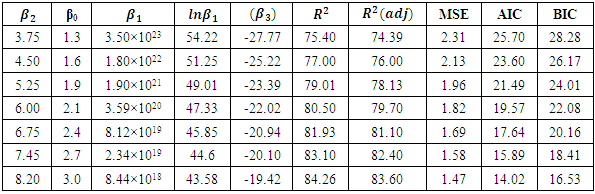
 from 0.3 to 0.25 and decrease
  from 0.75 to 0.10 in Table 4.3.Likewise, Table 4.3 below shows the values of the intercept and other parameters estimates with R2, Mean Square Error, AIC and BIC for various iterations. When
  increase by 0.25 and
  increase by 0.1.
|
 increase 0.1);
  increase 0.25)
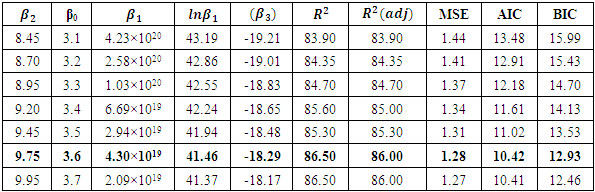
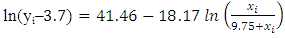 Hence, the identified Hill growth model is
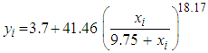
5. Conclusions
- The Hills Growth Model is nonlinear, then logarithmic transformation was applied to make the linear model paved way for its estimation of parameters. The study was able to show an alternative method of estimating the Hill Growth Model parameters using a real data set. A suitable Hill growth model was determined using Mean Square Error, R-Squared, Akaike Information Criterion (AIC) and Bayesian Information Criterion (BIC). The results of the sum of squared residual, R-Squared, AIC and BIC showed that the identified Hill Growth Model is adequate and can be used for forecasting of the amount of transmitted voltage against time.