-
Paper Information
- Paper Submission
-
Journal Information
- About This Journal
- Editorial Board
- Current Issue
- Archive
- Author Guidelines
- Contact Us
International Journal of Statistics and Applications
p-ISSN: 2168-5193 e-ISSN: 2168-5215
2020; 10(5): 118-130
doi:10.5923/j.statistics.20201005.02
Received: Sep. 11, 2020; Accepted: Sep. 30, 2020; Published: Oct. 15, 2020

Determinants of Under Five Child Mortality from KDHS Data: A Balanced Random Survival Forests (BRSF) Technique
 Abstract
 Reference
 Full-Text PDF
 Full-text HTML
Hellen Wanjiru Waititu1, Joseph K. Arap Koskei1, Nelson Owuor Onyango2
1School of Physical and Biological Sciences, Moi University, Eldoret, Kenya
2School of Mathematics, University of Nairobi, Nairobi, Kenya
Correspondence to: Hellen Wanjiru Waititu, School of Physical and Biological Sciences, Moi University, Eldoret, Kenya.
| Email: |  |
Copyright © 2020 The Author(s). Published by Scientific & Academic Publishing.
This work is licensed under the Creative Commons Attribution International License (CC BY).
http://creativecommons.org/licenses/by/4.0/

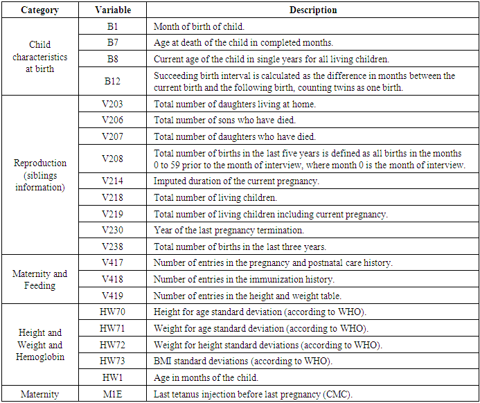
This study aimed at identifying the determinants of Under Five Child mortality (U5CM) based on Kenya Demographic and Health Survey (KDHS, 2014). One of the key challenges with Demographic and Health Survey datasets involves extreme imbalance between the mortality and non-mortality classes. In this particular research only 6.4% of children experienced under five years mortality while 94.6% survived beyond five years. To establish the determinants of U5CM, we opted to handle the class imbalance using four different balancing techniques: Random Under-sampling, Random Over-sampling, Both-sampling, and Synthetic Minority Over-sampling technique. We then did variable selection using Random Survival Forests following the four techniques. The variables selected from each of the four datasets were then used in a Cox-PH regression to determine the effect of select covariates on child mortality, after conducting appropriate model diagnostics. After the analysis, the variables which resulted in increased hazard of child mortality include V206 (Sum of demised sons), V207 (Sum of demised daughters), V203 (Sum of daughters living at home), V218 (Sum of existing children), V238 (Number of deliveries in the last 3 years), HW72 (Weight for height standard deviations) and interaction between B1 (Child’s Month of birth) and V206. Based on model selection indices,Under-sampling balancing schemes performed well for identification of U5CM determinants. By grouping these variables, this study identified birth characteristics of the child (such as age at birth), reproduction factors of the mother (such as number of siblings born before), feeding conditions and anthropometric measurements as key determinants of U5CM.
Keywords: Under five mortality, Balanced Random Survival Forests, Class Imbalance in data, Cox-PH regression in Survival analysis
Cite this paper: Hellen Wanjiru Waititu, Joseph K. Arap Koskei, Nelson Owuor Onyango, Determinants of Under Five Child Mortality from KDHS Data: A Balanced Random Survival Forests (BRSF) Technique, International Journal of Statistics and Applications, Vol. 10 No. 5, 2020, pp. 118-130. doi: 10.5923/j.statistics.20201005.02.
Article Outline
1. Introduction
1.1. Background
- The desire to understand the determinants of Under 5 Child Mortality (U5CM) poses a very important aspect of research, as countries aim to achieve the Millennium Development Goals (MDG 2015 – 2030). The Demographic and Health Surveys (DHS) program has been very instrumental for obtaining and disseminating authentic, national representative data on family planning, fertility, maternal and child health, among other health issues. The most recent DHS survey conducted in Kenya was KDHS 2014. This study aims at identifying the determinants of U5CM in Kenya. Comparisons shall be made between mortality and non-mortality groups from the KDHS 2014 data. Mortality group composes a very minority class (less than 7%) of the entire population, while the non-mortalities constitute the majority class. Imbalanced classification is a common problem with most datasets including mortality data, fraud data, fraud detection, claim prediction, default prediction, spam detection among others. Handling imbalanced classification has received prominence in many studies ([1], [2], [3], [4], [5]). The KDHS data is associated with 1,099 variables and 20,964 rows of data. Due to high dimensionality of the data, one needs to identify effective variable selection techniques in order to handle a problem such as to identify determinants of child mortality. Machine learning techniques (that require no distributional assumptions on data) such as Random Survival Forests, support vector machine among others have received wide application in studies involving high dimensional datasets ([6], [7], [8], [9], [10], [11], [12]). These machine learning techniques have been useful when dealing with problems such as missing data imputation, classification imbalance and variable selection. Besides, DHS data is often associated with missing data problem. This is often one of the main data analysis tasks before running the desired models. In this case, we did multiple imputation using RF algorithms, before proceeding with RSF classification. In this study however, we dwelt more on handling the challenge of imbalanced classification in mortality data.The remaining part of the paper is laid out as follows: Section 2 discusses the methodology employed in this study, from description of the data, exploratory data analysis, effects of data imbalance, the theory behind Random Survival Forests, the structure of the COX-PH model used, and finally model selection criteria using concordance statistic. Section 3 summarizes the results of the study both from variable selection using RSF to the Cox-PH fit. Finally, section 4 offers a discussion of our results against other ongoing research on determinants of U5CM.
2. Methodology
2.1. Data Description and Ethical Approval
- The data for this research was drawn from the 2014 Kenya Demographic and Health Survey (KDHS) data [13]. This is the sixth Demographic and Health Survey (DHS) conducted in Kenya since 1989. KDHS is a national research undertaking conducted every five years with an intention of collecting a wide range of data with a strong interest on indicators of reproductive health, fertility, mortality, maternal and child health, nutrition and self-reported health habits among adults [14]. It is a household sample survey data with a national representation where households are selected at random from Kenya National Bureau of Statistics (KNBS) sampling frame.The survey procedures, instruments and sampling methods used in the KDHS 2014 acquired ethical recommendation from the Institutional Review Board of Opinion Research Corporation (ORC) Macro International Incorporated, a health, demographic, market research and consulting company situated in New Jersey, USA. We sought official registration on the DHS website and got permission to use the KDHS 2014 data. The data was downloaded in SPSS format and constituted 1,099 variables and 20,964 observations. Using package foreign, the data was imported to R software version 3.6 for analysis. Variables with 100% missing observations and those which were correlated were deleted from the data reducing the number of variables to 786. Survival time and status variables which are important considerations when analyzing survival data were calculated and included in the dataset.
2.2. Data Exploration and Analysis
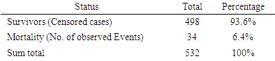
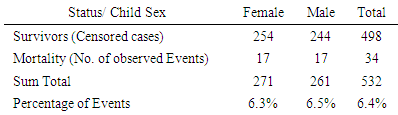
- The data was explored and analyzed using R software. This involved summarizing and visualizing characteristics of the variables within the dataset. The entire dataset was found to be highly imbalanced with the mortality class having 871 observations, constituting 4% of the overall data while the majority class had 20,093 observations constituting 96%. For this analysis, we singled out on the Nairobi dataset only from the KDHS (2014) data. Different covariates including region, residence, sex, level of education, wealth index, among others, were also found to have high class imbalance (between survivors and non survivors), with the minority class size ranging between 3% and 6%. The aim of this research is to find an effective way of applying the variable selection technique called Random Survival Forest (RSF), to analyze data with imbalance. KDHS data is a national survey data which is classified into 8 regions, constituting former provinces in Kenya. For this work, we analyzed data only for Nairobi region, being a unique urban system in Kenya. It’s a metropolitan region with improved health facilities and access, while also having high levels of socio-economic disparity among populations. Nairobi hosts some of the largest slam settlements of the world including Kibera, Mukuru, Mathare and Kangemi. However, majority of Nairobians are in the middle and upper class by socio-economic status classification enjoying sufficient access to proper health and nutrition for their children.In the KDHS 2014 data, Nairobi region alone was associated with 788 covariates and 532 observations. Some variables in this subset of data were found to have 100% missing information and others were highly correlated. These variables were deleted leaving 757 variables. Some of the variables that were deleted from Nairobi data include variables related to medication for fever that are currently out of use, for example ML15A (time when the individual began malaria drugs), ML15B (days when child took malaria drugs), ML15C (first source of fansidar), ML23C (first source for other anti-malaria) among others. Other variables like V000 (country code), V024 (De facto region of residence), among others were also deleted from Nairobi data set. The data was found to have high level of missing information. The algorithm “missForest,” which is a random forest-based algorithm for missing data imputation [15] was applied to handle missing data.Nairobi dataset equally showed high level of class imbalance. This imbalance between mortality and survivor classes is clearly shown on Table 1(a) with 6.4% minority class (mortality class) representation. Similarly, the variables in the data (covariates) show high imbalance in the mortality class. Table 1(b) shows the imbalance between mortality and survivor classes in one of the covariates – child sex.
|
|
2.3. Imbalance and Its Effects in Datasets
- A dataset is said to be technically imbalanced if its class distributions are not equal. However, when there is a significant, or in some cases extreme, disproportion among the number of examples of each class of the problem, then the dataset is said to be imbalanced [18]. For instance, in a cohort of 1000 children, its often the case that mortality group over the study period composes of less than 50 children (representing less than 5%) or less, hence leaving an entire 95% plus as the non-mortality group. Imbalanced data classes are common in many real-life situations including mortality data where the survivors greatly outnumbers the mortality, rare disease diagnosis data records where large number of patients do not have the disease, fraud detection, among others. In most of the imbalanced data situations, it is the underrepresented class which is of most interest, since despite its being rare, the minority class may carry important and useful knowledge required in prediction.When dataset is imbalanced and one class dominates the other, machine learning algorithms such as random forests among others have issues classifying correctly. The algorithms are sensitive to proportions of different classes. They often show biased behavior supporting the majority class and present the minority class lightly [16], [19]. This leads to higher rate of misclassification in the minority class samples [20], [21] which in turn results in weak predictive accuracy of the minority class and misleading high predictive accuracies in the majority class, as a result of correct classification [22], [23], [24]. Thus, the performance of such algorithms is decreases significantly when it comes to predicting the minority class.Many machine learning algorithms are designed to maximize overall accuracy. This can be misleading in imbalanced datasets because the minority class holds a small effect of this measure. However, when data is balanced, accuracy rates tend to decline [25]. This is attributed to the fact that balanced data reduces the training set size leading to degeneracy of the model through omission of cases encountered to the test set.The machine learning algorithms aim at minimizing the overall error rate instead of paying attention to the minority class. Therefore, they do not make accurate prediction for the minority class if they don’t get the necessary amount of information.[25] in his research demonstrating problems encountered when unbalance data is used in data mining algorithms found that algorithms tend to degenerate by assigning all cases to the majority class when data is highly imbalanced and still achieve high accuracy scores. Hence, evaluating algorithm performance using predictive accuracy alone is inappropriate when data is imbalanced. In order to overcome these issues it is important, when working with such machine learning algorithms to work with balanced classification. However, this is in most cases overlooked. We are therefore interested in construction of classifiers that are skewed toward the minority class, while still maintaining the precision of the majority class.
2.4. Data Balancing Techniques
- Various techniques have been suggested to solve problems associated with class imbalance. We can group these techniques into four categories, subject to how they deal with imbalance. The categories includes data level (or external/ re-sampling techniques), algorithm level (or internal) techniques, cost-sensitive learning techniques and ensemble-based methods. There is no open directive that indicates the best strategy to use. However, many studies have shown that, external techniques greatly improve the ultimate performance of the classification in comparison with non-preprocessed data set for various types of classifiers [18]. In addition, re-sampling techniques are independent of the classifier, can be easily implemented for any problem and do not need adaptation of any algorithm to the dataset [26]. They are also able to effectively balance the dataset resulting in training sets that are suitable for satisfactory calibration of machine learning algorithms [27]. [28], [29] and [16] have proved the effectiveness of balancing class distributions using data level techniques.In this research we apply the Data level Preprocessing (or external) techniques. The methods re-balance the sample space aiming to lessen the effect of the imbalanced class distribution in the learning process. The Data level techniques are further classified into three groups [30] which are: under-sampling methods, over-sampling methods and hybrids methods which combine both sampling methods. The Data level techniques used in this research are:a) Random under-samplingThis aims at balancing dataset by randomly eliminating examples of the majority class up to when the dataset is balanced. The major drawback of this method is that there is a high possibility of discarding potentially useful data pertaining to majority class leading to a possibility of information loss.b) Random over-samplingWhile the under-sampling method involves removal of samples from the majority group, over-sampling method generates new samples for the minority class. To balance the data using this method, the observations from the minority class are reduplicated. New instances are created from the existing ones; hence over-sampling does not increase information but raises the weight of the minority class by replication. One advantage of over-sampling methods is that there is no information loss. However, since over-sampling simply makes exact copies of the minority class observations, it increases the chances of over fitting due to replication. Therefore, even if there will be improvement in the training accuracy of the data the overall accuracy of the data may be worse. In addition, while dealing with large imbalanced data sets, over-sampling may increases computational work and execution time [31]. c) Both-samplingThis method combines both under-sampling and over-sampling methods by performing over-sampling with replacement on the minority class while the majority class undergoes under-sampling without replacement. d) Synthetic Minority Oversampling technique (SMOTE).This is a hybrid method in re-sampling techniques where both under-sampling and over-sampling approaches are combined with an aim to overcome their drawbacks. SMOTE has become one of the most outstanding approaches in data balancing field [18]. The key idea in SMOTE proposed by [32] is to produce new samples of the minority class artificially. This helps to avoid over fitting brought about by reduplication of minority class instances. Additionally, the majority class examples are under-sampled, giving rise to a more balanced dataset.Generation of Synthetic samples takes the following steps:• Randomly select a minority and its
 nearest minority class neighbors. The value of
  is determined by the amount of oversampling needed.• Calculate the difference between the vector of selected minority and that of one of its nearest neighbors.• The difference got is then multiplied by a random number between 0 and 1. The result is added to the selected minority vector. By so doing a new random point is added along the line joining the two vectors under consideration.SMOTE is thus implemented as follows. Let
  be the feature vector for the selected minority and
  be the feature vector of a randomly chosen neighbor. A new synthetic minority
  is generated in the feature space as:
 where
where  is a uniform random variable. An arbitrary point is selected along the line segment between two points under consideration. Thus, the synthetically generated data can be interpreted as a randomly sampled point along the line segment between the two minority samples in the feature space.In the R environment, Package DMwR [33] and ROSE package [34] are used to enhance data balancing. ROSE package [34] is used to enhance data balancing using under-sampling, over-sampling and both-sampling methods. On the other hand, package DMwR [33], assists in data balancing using SMOTE. In SMOTE the parameters
  and
and  respectively control the amount of over-sampling and under sampling to be done. If a completely balanced data set is required, the minority cases are doubled while the majority class is halved.In this study, we used under-sampling, over-sampling, both-sampling and SMOTE methods to balance the Nairobi region data. The balanced data was analyzed using RSF algorithm.
2.5. Random Survival Forest Algorithm
- The KDHS dataset has a total of 1099 variables that are possible candidates for predicting child mortality. After some data management exercise, the number of candidate covariates reduced to 757 possible covariates. Before fitting a regression type model in order to embark on the exercise of determining the effect of child mortality predictors, we needed to do a variable selection exercise in order to further reduce the variables of importance to a manageable subset of important variables. A Random Survival Forest technique, supplemented by our own intuition of sensible covariates for child mortality resulted into a reduced set of utmost 20 covariates for the regression steps that followed.Random Survival Forest algorithm is described as follows [35]:a) The procedure starts by randomly drawing
 bootstrap samples from the initial data consisting of
  samples. On average, each bootstrap sample sets aside 37% of the data called out of bag (OOB) data with respect to the bootstrap sample and each sample has
  predictors.b) For each of the drawn samples, a survival tree is grown. Construction of survival tree begins with randomly selecting
  out of
  possible predictors in
  for splitting on. The value of
  depends on the number of available predictors and is data specific. All the
  bootstrap samples are designated to the top most node of the tree which is also referred to as the root node. This root node is then separated into two daughter nodes each of which is recursively split progressively maximizing survival difference between daughter nodes/ increasing within-node homogeneity.c) Trees are grown to full size up to the point when no new daughter nodes can be formed due to the stopping criterion that the end node (most extreme node in a saturated tree) should have larger than or equal to
  unique events.d) After the tree is fully grown, cumulative hazard function (CHF) is computed as well as the mean over all CHFs for the
  trees. This is done to attain the ensemble CHF.e) By using out-of-bag (OOB) data only, the ensemble OOB error is calculated using the first
  trees, where
2.5.1. Node Splitting
- From the RSF algorithm, a forest originates from randomly drawn
 bootstrap samples. Each bootstrap sample becomes the root of each tree in the forest. There are
  predictors in each bootstrap sample. From the
  predictors, we randomly select
  predictors for splitting on. Suppose we take
  to be the
  node to be split into two daughter nodes. Within node
  , let there be
  observations each with survival time denoted by
  , and censoring status given by
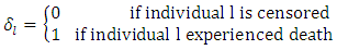 In right censored data, all details of developing a forest take into consideration the outcome. For right censored data, the outcome is survival time and censoring status [36]. The information at time
  can be summarized as in Table 2 below.
|

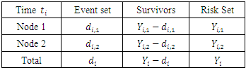
 stands for the number of events in daughter node
  at time
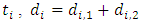
 represents individuals who are alive in daughter node j,
  at time
  ,
,  is the number of
 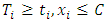 , where
  is the duration of survival for the
  individual and
  the distinct event time in node
 is the number of
 From the
  predictors in node
  take any predictor
  (for example age). Using predictor x, find a splitting value
  (for example from predictor age, the splitting value could be 2 years). The splitting value
  is chosen in such a way that the survival difference for predictor
  between
  and
and  is maximized.
  separates to the left node while
  goes to the right node. The survival difference between the two nodes is calculated using a predetermined splitting method. This procedure is repeated with another splitting value
  until we get a value which results in maximum survival difference in predictor
  . The same procedure is repeated for the remaining
  predictors in node
  This is done until we get predictor
  and split value
  which results in maximum survival difference between the two daughter nodes [37]. This process is repeated at every node. When survival difference is maximum, unlike cases with respect to survival are pushed apart by the tree. Increase in the number of nodes causes dissimilar cases to separate more. This results in homogeneous nodes in the tree consisting of cases with similar survival.Splitting criteria is one of the aspects of growing a tree. In this research, log rank splitting rule was used in splitting the node.
 2.5.2. Log Rank Splitting Rule
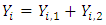
- The log-rank splitting rule separates the nodes by selecting the split that yields the largest log rank test. The log rank test is the most frequently used statistical test to compare two or more samples non-parametrically in censored data. PH assumption is the key requirement for the optimality of log rank test. For a split using covariate
 and its splitting value
  , the goodness of fit will be measured using log rank statistics represented as;
 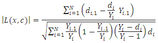 This equation measures the magnitude of separation between two daughter nodes. The best split is given by the greatest difference between the two daughter nodes which is given by the largest value of
  RSF gives a measure of variable importance (VIMP) which is totally nonparametric. In this study, using the RSF model, the highly predictive risk factors from the four balanced datasets were extracted. The extracted important predictors were then fitted in the Cox PH model in order to estimate the effect of statistically significant predictors.
2.6. Determining Predictors of Child Mortality
- The Cox ph model [38] is frequently used to determine collectively the effect of various risk factors on survival duration. The formula for the Cox ph model is written as
 This formula displays the risk at time
  for an individual specified by a set of covariates X. In this case,
  is a group of variables that are used in the model for prediction of the risk of the given observations. From the formula, the risk at time
  is a product of
  , the baseline hazard function and
  , the exponential to the sum of the
  predictor variables in
  . the baseline hazard function indicates what the risk would be when there are no covariates. The coefficient
  gives the magnitude of the influence of the covariates.
2.6.1. Checking the COX-PH Assumptions
- For appropriate use of the Cox proportional hazards regression model, there are several important assumptions that need to be checked.These include:• The proportional hazard assumption. Schoenfeld residuals were used to test this assumption.• Functional relationship between the log hazard and the covariates. Martingale residual were used to assess this assumption.• Possible presence of outliers or influential observations. Deviance residual was used to examine possible presence of influential observations.
2.7. Model Selection Criterion
- Comparison of prediction accuracy of the different models was done based on concordance index. In survival analysis, a pair of observations is said to be concordant if for the individual that got the event fast the model predicts a higher risk of event. Harrell’s concordance index (C-index) [39] is used to estimate prediction error. It estimates the likelihood that in a pair of cases selected at random, the case that came to have an event first had a worse predicted result. Suppose we have two observations whose outcome is predicted. If the observation predicted to have the worst outcome experiences an event first, then the two observations are said to be concordant (i.e. they have the appropriate practice). Computation of concordance error rate is as given below.a) The procedure begins by forming all potential pairs of observations from the entire data. b) A pair is omitted if:• The observation with shorter duration of survival is censored.• Duration of survival is equal for the pair but one or both observation is censored.c) After the omissions are done, we remain with all the other pairs which are referred to as permissible pairs.A score of value 1 is given to a permissible pair if:• For all pairs having unequal survival durations resulting in prediction being worse for the observation with shorter survival duration. • For all pairs having uniform survival durations resulting in similar prediction results.• For all pairs having equal survival duration given that not both observations are events, the observation with event results in a worse prediction outcome.A score of value 0.5 is given to a permissible pair if:• For all pairs having unequal survival duration, the prediction outcome is equal. • For all pairs having equal survival duration, prediction outcomes are not equal.• For all pairs having equal survival duration given that not both observations are events, prediction outcome is worse for the observation with censored results.If we denote the sum of all the permissible pairs as Concordance, then the concordance index, C is defined as
 The error rate,
  is given by
  where
where  .
.  indicates perfect accuracy while
  is equivalent to random guessing.
3. Results
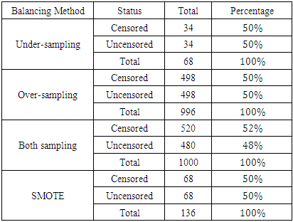
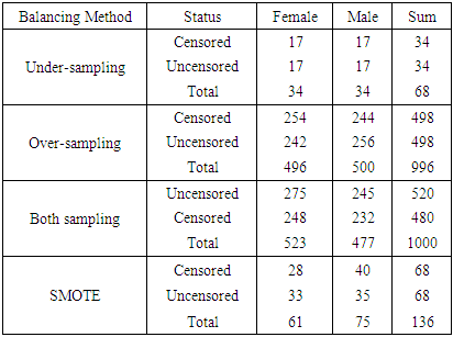
3.1. Balancing Schemes
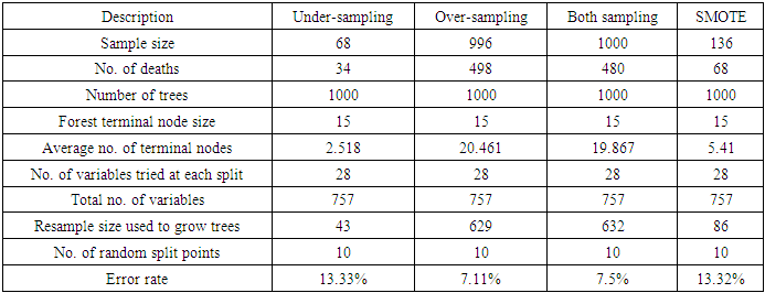
- The sample sizes obtained after different balancing methods are shown in Tables 3(a) and 3(b)
|
|
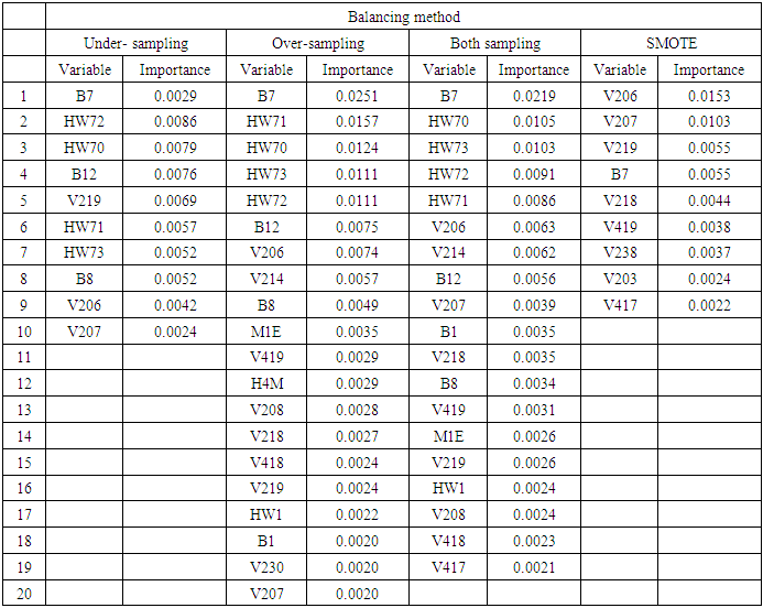
3.2. Variable Selection Using RSF after Different Balancing Schemes
- From the results in table 4, a forest of 1000 trees was grown for each data set. This was done by drawing 1000 bootstrap samples from the respective initial data with the sample sizes given in the table. The size of each bootstrap sample drawn is given as resample size used to grow trees in table 4. The bootstrap samples are of different sizes depending on the sample size of the initial data and the balancing method used. Each of the 1000 bootstrap samples is designated to the root of the tree. To develop each tree, 28 out of the 757 possible predictors are selected at random for splitting. The root node is then split into two daughter nodes each of which is recursively split progressively maximizing survival difference between daughter nodes. Node splitting continues until each tree if fully grown. This is achieved when the most extreme node has no fewer than 15 different events. This implies that the samples with bigger number of events will form bigger trees. Hence, the more the number of events, the bigger the average number of terminal nodes and the smaller is the error rate. Over-sampling method with the biggest number of events has the smallest error rate while under-sampling method with the smallest number of events has the highest error rate. Even though the sample sizes are different, the number of variables in the four samples is the same. This explains why the number of variables tried at each split and the numbers of random split points are equal in the four samples.
|
|
3.3. Determining the Variable Effects
- In order to measure the effects of the selected variables on child mortality, we fit a Cox PH model on the covariates from each variable selection exercise. Before the predictors are fitted in the Cox model, ph assumptions were tested.
3.3.1. Testing Cox Proportional Hazards (PH) Assumptions
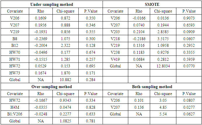
- Table 6 displays the results of proportional hazards assumption. The global test gives a general picture of proportional hazards violations among the variables in the model. Therefore, p.value < 0.05 suggests one or more violations. For variables that do not satisfy the assumption, interaction with time varying covariate is included. Variables that finally do not satisfy the assumption even after interaction with time varying covariate are not supposed to be included in the model.
|
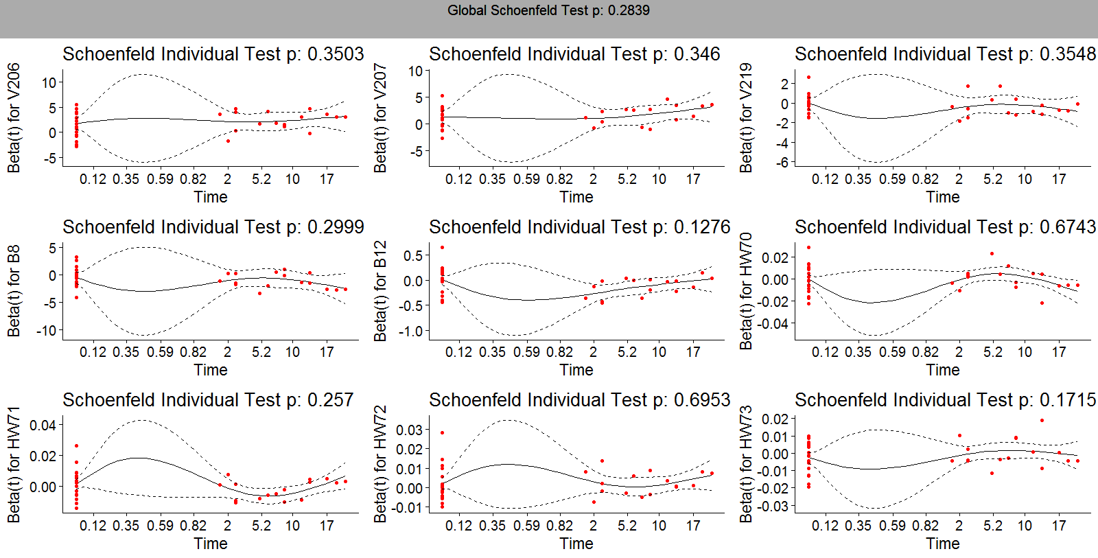 | Figure 1. Schoenfeld residuals for variables in under sampling method |
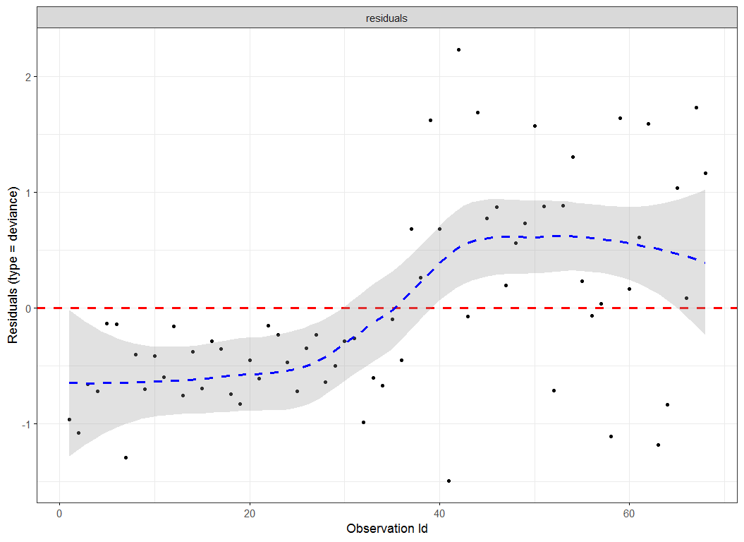 | Figure 2. Deviance residuals for under sampling method |
3.3.2. Parameter Estimates
- From the previous section, we noted that the different balancing methods yielded different sample sizes and different predictors from the RSF classification. After diagnostic tests on Cox PH models, the respective predictors were fitted to the parsimonious Cox PH model [37] in order to check concurrently the effect of different risk factors on survival time.The results of fitting the Cox model are shown in Table 7. The regression coefficient column marked “Coefficient” gives estimates of the logarithm of the hazard ratio between the two groups. From the estimates, a positive coefficient is said to increase the risk of death (hazard) and thus decrease the expected (average) survival time. On the other hand, a negative coefficient reduces the risk of death and thus raises the expected survival span. In explaining the determinants of child mortality, one therefore is interested in the variables with positive coefficient, which are positively related with the event (mortality) probability, and consequently negatively related with the length of survival. From table 7, under-sampling method resulted in 9 predictors, out of which only 3 were likely to increase the risk of death. Similarly, SMOTE returned 5 predictors that are likely to increase the risk of death out of 7 important variables which satisfy PH assumptions. Over-sampling and both-sampling method had 3 and 2 predictors respectively all of which had positive coefficients.
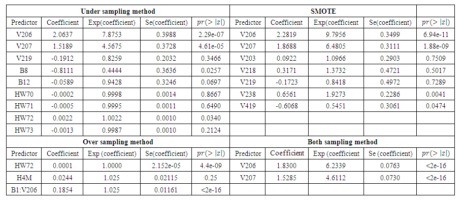 | Table 7. Result of fitting the respective predictors in Cox PH model |
 predictor increases (for continuous type covariates), the event hazard increases and thus the length of survival decreases.From table 6 for example, variable V206, in under-sampling method has
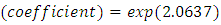
 . HR value which is clearly greater than 1 implies that variable V206 increases the hazard by a factor 7.8753. This is deduced from the fact that a predictor is related with increased risk when the value of HR>1, and decreased risk when HR<1. When the HR value is close to 1, the predictor has no impact on survival. From our results, there are 2 predictors in under-sampling method associated with increased risk, 0 in over-sampling, 2 in both-sampling and 4 in SMOTE (refer to Table 6 above).The column marked
  gives the value of the Wald statistic. Wald statistic evaluates whether the explanatory variables in a model are significant. A variable is said to be statistically significant when its p.value is less than 0.05.
3.3.3. Model Goodness of Fit Statistic
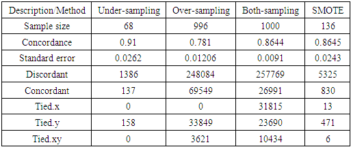
- The concordance statistic was used to analyze the performance of the models on prediction of mortality. Concordance values are given in Table 8 below.
|
4. Discussions
- The study attempts to understand the determinants of under five mortality using survey data from DHS. In this case, Kenya DHS survey 2014 dataset was used for the analysis. The dataset (after variable cleaning) is composed of 757 variables that are candidate determinants of Under five Child mortality. This poses a problem of variable selection from such high dimensional datasets preceding a proper analysis in which the intention is to explain variable effects. Besides, there is too much class imbalance in the datasets particularly where interest is to compare mortality and non mortality groups. For instance, 6.4% of children experience mortality while 93.6% survived up to the age of 5 years. This imbalance is too huge that a direct comparison (before balancing) between two such groups is likely to yield biased results.Two challenges were addressed in this study. One problem involved trying to balance the dataset classes before making comparisons between mortality and non mortality cases. The other challenge was due to variable selection. One needs to conduct a proper variable selection exercise in order to identify the correct set of variables to use for the regression analysis. Most studies explore determinants of child mortality using DHS survey data. [6] used Uganda 1996, 2000, 2006 DHS dataset, [7] used Uganda 2011 DHS, [8] analyzed the data from complete birth histories of four Nepal Demographic and Health Surveys (NDHS) done in the years 1996, 2001, 2006 and 2011, among many other studies. In this study, we have also tapped into the richness of KDHS (2014) dataset, to establish the determinants of U5CM. The key improvement over many studies that have used DHS data to answer the same question lies in our choice to ensure the following remedies are done: (i) class imbalance is eliminated before comparisons are done, (ii) imputation for missing data is done using a machine learning approach (the missForest package in R software used), (iii) variable selection is accomplished again using a machine learning algorithm (RSF). In most studies, researchers often use self intuition or previous studies to determine which covariates to add to their regression models. All these remedies were done before applying a Cox PH regression on the data to reduce chance of reporting biased findings. Many studies commonly employed regression techniques to explore the determinants of U5CM. Cox PH regression was used by [6], [7], [8] among others. Although we also used the Cox PH model, we preceded it diagnostics including multiple imputation, classification balancing, variable selection, and Cox PH assumptions tests, to ensure that the results from the Cox PH are more reliable. Our findings show that child mortality is associated with variables related to: child characteristics at birth (such as age at birth), reproduction factors of the mother (such as number of siblings born before), feeding characteristics and anthropometric measurements. This is in line with other findings such as [6] who used Cox PH regression and established that region of residence, sex of the child, type of birth (multiple), birth interval (less than 24 months after the preceding birth), and mother's education were related with an increased risk of children mortality before their fifth birthday. [7] also established that factors related to mother characteristics and previous births such as sex of the child, sex of the head of the household and the number of births in the past one year was found to be significant. [8] explored the effect of mother’s education, child's sex, rural/urban residence, household wealth index, regions ecological zones and development. It’s worth to note that even though most of the studies that rely on DHS datasets ([6], [7], [8]) are challenged with high dimensional data and a variable selection dilemma, there is no mention of any statistical form of variable selection. DHS datasets typically are composed of over 700 variables that are candidate determinants of child mortality and one need to carefully select which variables to include in the resultant regression type models. Majority of the studies explore the effect of a predetermined, select group set of covariates, based on self intuition or variables explored from previous studies. We attempted to do a variable selection using a machine learning algorithm, before subjecting the selected variables to Cox PH regression. Other than finding the determinants of under five mortality, different data balancing methods were used and model selection done using concordance index. In their research [40] used SMOTE to balance data before integrating it with RSF. In this research, under-sampling method resulted in a better model with a concordance index of 0.91 as compared to other balancing methods used. SMOTE generates synthetic samples along the line segment joining two minority samples. By so doing there is a tendency of generating a decimal value in factor or numeric variables which are not meant to be in decimal form. In as much as under-sampling method may discard potentially useful data in majority class there is no loss of data in the minority class which is our main class of interest.
5. Conclusions
- In this research, we presented a framework for determination of under five child mortality using the 2014 KDHS data. The framework involved data balancing, variable selection using RSF method and variable prediction using Cox PH model. Various challenges and effects of working with imbalanced data are discussed in this research as well as the various data balancing methods. Analysis of four data balancing methods; over-sampling, under-sampling both-sampling and SMOTE techniques was conducted where under-sampling model emerged the best with a concordance index of 0.91. Based on this research, child mortality is associated with variables related to child characteristics at birth (such as age at birth), reproduction factors of the mother (such as number of siblings born before), feeding characteristics and anthropometric measurements.