-
Paper Information
- Paper Submission
-
Journal Information
- About This Journal
- Editorial Board
- Current Issue
- Archive
- Author Guidelines
- Contact Us
International Journal of Statistics and Applications
p-ISSN: 2168-5193 e-ISSN: 2168-5215
2020; 10(4): 85-102
doi:10.5923/j.statistics.20201004.02
Received: July 30, 2020; Accepted: August 15, 2020; Published: September 5, 2020

Comparison Fuzzy Time Series -Clustering Applications in Production and Consumption Electric Prediction
 Abstract
 Reference
 Full-Text PDF
 Full-text HTML
Mohammed Eid Awad Alqatqat, Ma Tie Feng
Department of Statistics, Southwestern University of Finance and Economics, Chengdu, China
Correspondence to: Mohammed Eid Awad Alqatqat, Department of Statistics, Southwestern University of Finance and Economics, Chengdu, China.
| Email: |  |
Copyright © 2020 The Author(s). Published by Scientific & Academic Publishing.
This work is licensed under the Creative Commons Attribution International License (CC BY).
http://creativecommons.org/licenses/by/4.0/

This study aim to Comparison in fuzzy time series and fuzzy time and clustering and Proposed Method in the field production and consumption electric, the basic idea of three methods is to predictive the Possibility of future production and consumption electric based on historical data of production and consumption electric in the past, Nevertheless, Three methods have a different approach in transforming the value of production and consumption to the range of the random variables (the states). This paper considered the production and consumption data of electric in china from January, 2015 to December, 2019. The accuracy of three methods is verified by using the Mean Absolute Deviation (MAD), Mean Absolute Percentage Error (MAPE), the result shows that the Proposed Method has smaller MAPE, MAD, From fuzzy time series and fuzzy time clustering methods.
Keywords: Fuzzy time series, Clustering algorithm, Time Series, Prediction, Electric Energy
Cite this paper: Mohammed Eid Awad Alqatqat, Ma Tie Feng, Comparison Fuzzy Time Series -Clustering Applications in Production and Consumption Electric Prediction, International Journal of Statistics and Applications, Vol. 10 No. 4, 2020, pp. 85-102. doi: 10.5923/j.statistics.20201004.02.
Article Outline
1. Introduction
- Predicting the size of any phenomenon in the future is an important matter that helps in understanding the behavior of the phenomenon with time, and thus how to confront it. It is not possible to make future plans to confront the phenomenon except with its future dimensions and knowing the shape of these dimensions and their patterns. The consumption of electrical energy and its production within society has a dynamic character because it is not fixed, as it is affected by many variables, including the development of life and the increase in the necessary electrical appliances used in a necessary manner. So the scale of the problem is that electricity consumption and production now will not be the same after twenty years, for example.To face this problem, it is necessary to make estimates that monitor its size in the coming years, as it is not possible to build long-term plans to address this problem without making quantitative expectations for the size of the problem.The historical pattern of the problem can only be determined by the quantities that express its variables, as well as the increasing demand for electrical energy as a result of the development taking place in all facilities of life (industrial, educational, health and agricultural).The idea of this paper aims at how to build and fit a model to find the best model in a way that can accurately predict the rates of consumption and production of electricity for the coming years.Technological advancement, population growth and increased economic activities have led to a rise of various issues in the planning of energy such as investment, allocation as well as search for a new sustainable source of energy [1]. With electricity being the most formidable and reliable source of energy at the moment, more advanced use for it as well as its increased development and advancement is in consideration [2]. As a way of resolving these rising issues, there is an importance of having a central unit under which all this advancements are monitored, controlled as well as optimized to ensure that the generation and transmission of energy is uniform and most of all safe. Such control should be provided for by the power generating companies or the government. Such a system can help in automatic obtaining of the load data from networks of retail stores, factories, as well as office buildings which can then be self-diagnosed after which a trend analysis can be conducted to help perform a forecast on such data accordingly [3]. Such forecasting can be of use to the electric utility to help in the making of vital decisions such as decision to purchase or generate power, development of infrastructure as well as switching the load. Forecasting can be described as an approach that’s predictive analytical. Such an approach helps to deal with the prediction of the future through the use of past data as well as models [4]. The approach can also be used in different domains such as personal management, finance management, resource management and organizational management. Globally, the study of electric load forecasting management is still ongoing [5]. Most of the entities more concerned with such research are the electricity producing companies. Such studies help in making and determining how energy is going to be managed and planned by these firms. However, there are some methods that are already in place being used to forecast electricity. They include regression time series analysis, time series, autoregressive integrated moving average (ARIMA), artificial neural network (ANN), particle swarm optimization (PSO), Cluster analysis and the fuzzy time series (FTS) [6]. The cluster analysis and the FTS are the commonly used methods in forecasting since they can easily identify structures within data [7]. FTS uses different models which have been proposed by researchers to help in resolving problems. Some of the fields which use FTS include the enrolment of universities, stock prices index, financial sectors, evaluation of temperature and also electricity load consumptions [8]. The models used in FTS helps in the production of rules, systems and procedures used in forecasting which are all based on factors such as interval length of discourse universe, the weight of fuzzy relationship as well as the mathematical models [9]. These factors help in the determination of in-out sample forecasts. In order to achieve high levels of forecasting, the three factors are crucial for FTS [10].
1.1. Statement of the Problem
- The problem is the increase in consumption of electrical energy over time, therefore it is necessary to know the variables that affect the consumption of electrical energy and then study the possibility of finding projections of demand for electrical energy.
1.2. Objectives of the Study
- 1. Learn about the trend of electricity production and consumption trend.2. The importance of the role of the forecasting process in rationalizing decisions and exploring possible Consequences, defining the time series method and its effectiveness in the long-term forecasting process.3. Building mathematical models that can predict the quantities of electricity consumed and produced per month based on accuracy criteria.
2. Summary of Literature Review
2.1. Review of Fuzzy Time Series
- The regular set (crisp) is defined as a set of elements that is an item that can belong to or belong to a group and that the group may be specified or not defined [11], [12].Whereas, the set fuzzy group [13], Is that it is a class of elements with an organic degree and that this group is distinguished by an organic function that allocates each An element of a membership degree whose range is between zero and one, i.e. when the element takes a membership degree (1), this means that the element belongs entirely to the fuzzy group and when the membership degree is (0), this means that the element belongs absolutely to the group and other degrees vary between zero and one, when The degree of membership is (0.5), this means that the element belongs to the ratio (0.5) to the fuzzy group and does not belong to the group with the same percentage. The element belongs to the fuzzy group and does not belong to it with a ratio of (0.1) and this is closer to membership than to whether or not.Other researchers have provided many definitions of the fuzzy group, as Kaufmann knew it (1975) as follows [14], The fuzzy group is the group in which there are precisely clear boundaries between those elements that belong to it and those to which they belong. As for the definition that he provided in 1988 by Zimmerman [15] then the most accurate definitions are as follows: If X is a group of elements symbolized by generally denoted by x, the A group in A x is a set of arranged pairs, Is the membership function x in A which is a function from X to µ as µ A µ to where (x) the continuous membership field in the closed period.Fuzzy set has 2 attributes, namely:1. Linguistics is the naming of a group that represents a situation or certain conditions using natural language, such as: cold, cool, normal, warm and hot.2. Numerical is a value or number that indicates the size of a variable such as: 40, 25.50 and so on.There are several things that need to be known in understanding fuzzy systems, namely [16]:1. Fuzzy variables are variables that are to be discussed in a system fuzzy. Example: age, temperature, sales, demand and so on.2. Fuzzy set is a group that represents a certain condition or condition in a fuzzy variable. Example: Age variable is divided into 3 fuzzy sets, namely YOUNG, PAROBAYA and OLD. Variable the temperature is divided into 5 fuzzy sets namely COLD, COOL, NORMAL, And WARM and HEAT.3. Universe of Talk The universe of speech is the whole value that is allowed to be operated in a fuzzy variable. The universe of speech is a set of real numbers that always rise monotonically from left to right. Talking universe values can be positive and negative numbers.4. The fuzzy set domain is the whole value that is allowed in the universe of speech and may be operated in a fuzzy set. Like the universe of speech, the domain is a set of real numbers that always rises monotonically from left to right. Domain values can be positive or negative numbers.Literature done by Silva and Lisboa indicates that FTS model was introduced about two decades ago [10]. Since then, FTS has been used widely due to itsSuperiority while dealing with knowledge that is imprecise such as linguistics in regard to decision making [10]. Literature also indicates that there is need for the improvement of FTS forecasting which has been done through proposing new methods [17]. Since its discovery, FTS approach has undergone some modification leading to improvement to near perfection such as Song’s approach which offered a simpler forecast method in 1996 [18]. Some of the main issues with the FTS in regard to forecasting is the interval length which greatly affects the accuracy of the model [9]. Some of literature has addressed the problem through adjusting the interval lengths using an optimizing or distribution technique [19].Other researchers have focused on improving the weighted forecast models as a way of improving the accuracy of forecast results. This model is responsible for chronological order and various recurrences [20]. Further literature indicates that there are many forecasting models which are original and based on FTS, which are presented as well as combined with novel algorithms and technologies. Some of such models according to Chen include a model proposed by Singh who proposed that FTS can be used to forecast methods of crop production based on different parameters of computational methods [4]. Research done by Lee and Hong indicates that several models of FTS such as genetic algorithm, the simulated annealing algorithm can help forecast temperature [2].Research done by Ismail, Efendi and Deris indicates that the energy system in our case electricity has two aspect that is, supply and demand, since it is considered to be a product that has value [3]. Before 1960, the management of energy was concerned with prior aspect while the latter considered being a given data hence promoting the narrative of arranging for adequate supply to ensure that demand is met and well satisfied [11]. In the 1970s however, the prices hiked which led to researchers, governments as well as utilities to begin an investigation to the problem which was more focused on demand [21]. Ismail, Efendi and Deris defined energy demand management as “a systematic utility and government activities designed to change the amount and/or timing of customer’s use of energy” [11]. These activities also according to the literature involve utilizing the energy resources effectively, ensuring reliable supply, ensuring that the energy resources are managed efficiently, conservation of energy, a combination of power and heat systems, renewable energy systems, energy systems that are integrated and more so power delivery systems that are independent [22]. Research done by Hong and Lee indicated that the management of demand constitutes planning, implementation as well as monitoring of energy utilization all of which are designed to ensure that the consumers are encouraged to modify their pattern and level of energy usage [11]. Chen and Hong indicated that, in the prediction of energy consumption and demand, fuzzy time series is the best model since it bases the prediction on the size of the population, the methods used as well as the forecasting horizons [4]. Literature by Yu also indicates that the FTS has been used to forecast energy consumption especially the forecasting regional electricity loads [23]. FTS is also used help in the reduction of load forecasting error in short-term load forecasting problems [24]. Electricity producers and suppliers also use the FTS to estimate and predict the demand of electricity for monthly and seasonal changes.Research done by Ozawa and Niimura indicated that FTS has been used in countries such as Turkey to forecast short-term gross annual electricity demand by simply taking into consideration the political and economic as well as the electricity market conditions [5]. These are the same factors that are considered for any form of good which follows the rules of demand and supply. The two researchers also indicated that FTS is usually used or rather implemented while conducting research of fuzzy neural network for monthly demand of electricity forecasting as well as while using neural networks which helps in analyzing of several approaches while predicting the consumption of natural gas in different regions [25]. Countries such as Poland and Taiwan have gone on record as users of these models while using FTS. The FTS concept according to literature is a new approach which was developed through resolving problems of linguistic time series data [26]. FTS is an approach that uses a combination of linguistic variables and the analysis process of applying fuzzy logic into time series to help in solving data fuzziness [27]. Literature by Bolturk, Oztaysi and Sari indicated that FTS has an important aspect which is the assumption in regard to data which is not needed [6]. This assumption helps to differentiate FTS from other statistical approaches.
2.2. Review of Cluster Analysis
- After the person discovered that there are common characteristics in the parts of knowledge about me by classifying them, and philosophers and thinkers made efforts to lay the foundations and systems for this classification, and thus the word "classification" in the language is to distinguish things from each other in a way arranged in classes or sections and if arranged and known, it has been prepared A kind of classification system. Accordingly, classification can be defined as the process of grouping similar things together and all members of the first group, department, or single class resulting from classification participate in at least one specific characteristic that members of departments or other classes do not have to benefit from in scientific fields [28].It is known that classification methods are divided into two main groups of techniques, which are cluster analysis and discriminatory analysis. Cluster analysis is one of the techniques without supervision, where information about the classification group is little or no, and the goal is to find groups of data. Places of discriminatory analysis are an organic relationship in the pool of training samples and the main purpose is to build an appropriate classification rule for unknown new samples.Cluster analysis [29], [30]. Is one of the methods of analysis of multiple variables, and according to this analysis is the division of data into groups (clusters) that have scientific meaning and significance. The cluster analysis is often a step to enter into another analysis that carries goals that depend on the classification of data into clusters that bear the importance of research in the researcher example it summarizes the data. Regardless of whether it is the beginning of a subsequent analysis or classification of data, cluster analysis includes many scientific uses in various fields and disciplines. The concept of this analysis allows with many of those singular or viewed within a specific cluster that bear close characteristics to the characteristics of observations or data within the regular cluster to it, while those characteristics differ for projects with the characteristics of observations or data in other clusters.Clustering analysis depends on mathematical methods and algorithms in the classification process that have the ability to determine the extent of homogeneity between the classification vocabularies or the extent of inconsistency between its properties, and then give the researcher an opportunity to explain it within the laws and methods of cluster analysis. A cluster analysis is a grouping of community units or individuals in order to discover data structure. As individuals within one group are close or seen from one another, but they differ from individuals in other groups, as the results of the cluster analysis provide a known structure that can be used to make hypotheses to interpret the observed data. The cluster analysis which is described as the task of grouping a set of objects in a certain way hence forming a similar group referred to as a cluster is also used in relation to consumption and production of electricity. Literature indicates that cluster analysis has been introduced to help in analysis of electric production and consumption since the invention of smart grid. Advancement of technology has increased the demand of electricity hence forcing producers to scale up production. As such technology which considered more efficient and fast is usually used to ease and perfect the production and consumption. The smart grid was introduced into the energy sphere with the vision of producing and distributing low-carbon electricity more efficiently and reliably. As such, the consumers would be in apposition to manage their use through regulating their usage. In return, costs to both the consumers and the suppliers would be minimized. Through introduction of the grid, real time communication between the grid operator and the end consumer would be in real time which was intended to help flatten the electricity loads during pick hours. The process also was intended to help increase the options to the end user hence increasing the chances of optimizing the system. According to Rodden and Spence, this idea was referred to as smart load management by the end-user which was proven to be effective. This effectiveness was due to the cluster analysis which according to literature by Anderson its activities are based on those that are reported in time-diaries [31]. Clustering analysis helps or rather allow for assumptions that are empirically grounded in regard to flexibility that is potential [12]. Further literature also indicates that it helps to accurately predict flexibility of customer’s behavior. The cluster analysis according to literature is based on actual usage of appliances such as washing machines, cooking equipment’s, television sets and many more, it also based on collected activities from the time-diaries [32]. The data collected is usually based on reported activities in real time sequence of how the appear on the time-diaries rather than inferring flexibility indirectly from the load profiles or the time use average values. The end part is the assignment of data to the electric appliances to help in the characterization of the aggregate activity patterns.A survey done by Europe Statistics Group indicates that, there is one way in which consumers patterns can be traced which is through the use of data from their time-diaries [23]. This is where the consumer record the activities they are engaged in on daily basis in a certain sequence. The clustering approach therefore involves using the activity sequence deduced from the time-diaries of the consumers [34]. The analysis will then take into consideration the presence of any clusters basing on the similarity of the data gathered. The cluster analysis is used to group the consumers according to their performing activities by using similar timing as well as the duration to assist in the estimation of how the consumers consumes electricity. Some of the activities commonly used include cooking, watching a TV and doing laundry [35]. Research indicates that the consumption of energy is intertwined with people’s ways of life and also it is closely associated with how people act at various times of the day and seasons [36]. Cluster analysis in this research helps to determine the time the activities take place and how long they take. As such, the clustering analysis is done for the consumers who are clustered into different socio economic classes. Anderson’s research indicates that the lives of consumers are analyzed and described through and explicit reveal of the timing of energy-consuming activities [12]. Anderson is said to introduce new approach of the cluster analysis in this research through raising questions such as whether there are flexible users, and whether or not activities are moveable [12]. Research done by Nicholls and Strangers indicated that, when cluster analysis is done based on activity rather than the consumers, energy consumption in regard to activities causing it vary over the day rendering the approach irrelevant [37]. In the perspective of policies, when the time shift is targeted while analyzing electricity consumption, different groups will be affected differently hence eradicating the possibility of clustering [38]. However the policy means will have to depend on what it is aimed for concerning the flexibility of electricity usage [34] Clustering in our case is considered effective if individuals adapt to a shift in consumption of electricity from daytime to evenings as compared to vice-versa since the normal patterns are people use more electricity while at home during the evening hours [39]. Clustering is easier while considering consumers since people are easy to predict. People for example prefer to do some things at certain times.Which can be confirmed by the aggregate activity patterns as indicated in Anderson’s research [12]. For example, Anderson conducted a simple survey from which he observed that, during the time, people in New York preferred to do laundry during weekends and at lunch times [12]. However, this data had to be verified to determine its flexibility and whether there is need for complementary methods to verify the validity of the information for future reference [40].The cluster analysis helps to observe each activity at a time through isolation. The analysis also helps to evaluate whether the activities affects each other. For example, does cooking affect washing or TV time? Does consumption behaviors affect production and if so how? Research by Shove indicated that it is vital to collect the practices that constitute assemblages [41]. Clustering also helps establish the flexibility of the cluster activity by observing the actions of the individual before and after an activity [42].Individuals or rather consumers are interrelated hence affecting the flexibility and the context of their daily activities. As such, it is important to synchronize and allow time-space coupling between consumers from the same household. To encourage a time-space coupling, data should be collected from each and every consumer even if there are multiple users from one household [43]. Research done by Strengers indicates that the flexibility of a household in regard to energy consumption is related not only to adults but also to everyone in the household including the pets hence determined by the interaction of everyone in the household not excluding animals.
3. Methods
3.1. Fuzzy Time Series Method
- The use of fuzzy time series has been used to predict student registration data at the University of Alabama. The concept of fuzzy time series is proposed based on fuzzy set theory, fuzzy logic and approximate reasoning (Song and Chissom, 1993) [18]. Forecasting with fuzzy time series methods can capture patterns from past data to project future data (Song, 1993b) [19], better performance in forecasting real problems.The various definitions and properties of fuzzy time series forecasting are summarized as follows:Definition 1: Fuzzy set is an object of classes with a set of membership values. Suppose U is the universe of discourse,
 Where
Where  is a possible linguistic value of U then a fuzzy set
  linguistic variable of U is defined by equation 1 following:
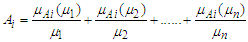 | (3.1.1) |
 a membership function is fuzzy set
  so
so If the membership is from
  to
to  is the degree that is owned by
  against
  .Definition 2: Let Y (t) (t =..., 0,1,2,...) subset
  , become a universe discourse with the fuzzy set
  defined and F (t) is a collection of
  then F (t) is called fuzzy time series defined in Y (t) (t =..., 0,1,2,...). From this definition F (t) can be understood as a linguistic variable
  of the linguistic probability value F (t). Because at different times, the value of F (t) can be different, F (t) as a fuzzy set is a function.From time t and universe discourse is different at each time so Y (t) is used for time t (Song and Chissom, 1993).Definition 3: Suppose F (t) is caused only by F (t-1) and appointed with
  then there is Fuzzy Relations between F(t) and F(t-1) expressed by the formula
 | (3.1.2) |
 is the Max-Min composition operator. The relation R is called the first order model F (t).If fuzzy has relation R (t, t-1) of F (t). (t) Is time independent so for different times
 So that F (t) called time-invariant fuzzy time series.Definition 4: If F (t) is produced by several fuzzy sets
 Then the fuzzy relationship is symbolized by:
 Where
Where  And such relationships are called
  order fuzzy time series.Definition 5: Let F(t) is produced by F(t-1), F(t-2),…., and F(t-m)(m>0) simultaneously and the relation is time variant then F(t) called fuzzy time series and the relation can be expressed with a formula:
 | (3.1.3) |
 (T) and forecasting of production and consumption in the next month.Step 6: Defuzzifying the acquired outcomes or conversion of fuzzy values into qualitative values.
3.2. Fuzzy Time Series and Clustering
- The proposed clustering algorithm is used to partition universe of discourse into different lengths of intervals [43].Step 1: Sort the numerical data in ascending sequence,Shown as follows:
 Calculate the threshold value for stopping condition of the proposed clustering algorithm, shown as follows:
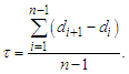 | (3.2.1) |
 Where the symbol “{}” denotes a cluster.Step 3: Assume that there are p clusters, calculate the cluster center cluster center k of each cluster k as follows:
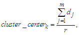 Where dj is the data in Cluster k, r is the number of the data in Cluster k, and 1≤ k ≤ p.Calculate the distance
  between any two adjacent cluster centers
 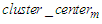 and
and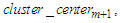 shown as follows:
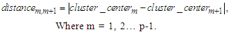 | (3.2.2) |
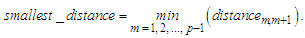 Step 5: If smallest distance
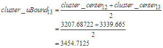
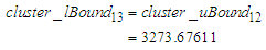
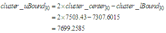
  then combine the clusters having the smallest distance between them into a cluster and go to Step 3. Otherwise, go to Step 6.Step 6: Calculate the upper bound
  of
of  and the lower bound
  of
of 
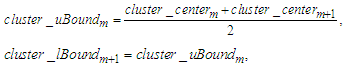 | (3.2.3) |
 of the first cluster and the upper bound
  of the last cluster can be calculated as follows:
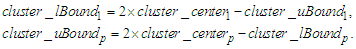 | (3.2.4) |
 form an
  , which means that the upper bound
  and the lower bound
  of the cluster
  are also the upper bound
  and the lower bound
  of the interval
  , respectively. Calculate the middle value
  of the interval
  as follows:
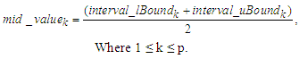 | (3.2.5) |
 obtained in Step 1, and then define linguistic terms
  represented by fuzzy sets, shown as follows:
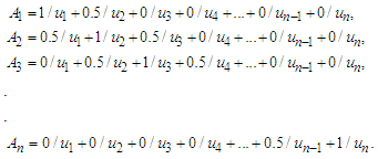 Step 3: Fuzzily each historical datum into a fuzzy set. If the datum is belonging to
  , then the datum is fuzzified into
  where 1≤ i ≤ n.Step 4: Construct the fuzzy logical relationship based on the fuzzified data obtained in Step 3. (Note: If the first order fuzzy time series is used and the fuzzified values of time t-1 and t are
  and
and  , respectively, then construct the fuzzy logical relationship
  where
where  are called the current state and the next state of the fuzzy logical relationship. If the nth order fuzzy time series is used and the fuzzified values of time t-n… t-2, t-1 and t are
  respectively, then construct the Fuzzy logical relationship
  where
where  are called the current state and the next state of the nth order fuzzy logical relationship). Based on the current state of the fuzzy logical relationships, let the fuzzy logical relationships having the same current state to form a fuzzy logical relationship group.Step 5: Calculate the forecasted output at time t by using the following principles:Principle 1: If the fuzzified values at time t-n… t-2, and t-1 are
  respectively, and there is only one fuzzy logical relationship in the fuzzy logical relationship groups, shown as follows:
 Then the forecasted value of time t is
  where
where  are the middle value of the interval
  and the maximum membership value of
  occurs at interval
  .Principle 2: If the fuzzified values at time t-n… t-2, and t-1 are
  respectively, and there is only one fuzzy logical relationship in the fuzzy logical relationship groups, shown as follows:
 Then the forecasted value of time t is calculated as follows:
 | (3.2.6) |
 denotes the number of fuzzy logical relationships
  in the fuzzy logical relationship group,
  and
and  are the middle value of the intervals
  and
and  respectively, and the maximum membership values of
  and
and  occur at interval uk1, uk2,…, and
  , respectively.Principle 3: If the fuzzified values at time t-n… t-2, and t-1 are
  and
and  respectively, and there is only one fuzzy logical relationship in the fuzzy logical relationship groups, shown as follows:
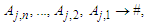 Then the forecasted value of time t is calculated as follows:
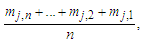 | (3.2.7) |
 are the middle values of the intervals
 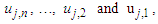 respectively, and the maximum membership values of
  and
and  occur at intervals
  and
and  respectively.
3.3. Proposed Method for Predicting Using Fuzzy Time Series and Clustering
- Through our studies Fuzzy time series and clustering Time series analysis is an important statistical topic that deals with the behavior of phenomena and their interpretation over specific periods. The objectives of time series analysis can be summed up by obtaining an accurate description of the special features of the process from which the time series is generated, building a model to explain the behavior of the time series and using the results to predict the behavior of the series in the future, in addition to controlling the process from which the time series is generated by examining what can happen when some change Form parameters. To achieve this, a thorough analytical study of time-series models based on statistical and mathematical methods are required.Our proposal includes the same previous steps Fuzzy Time Series and Clustering but we have specials steps and they are as follows:First Step: the data will take 60 months from January 2015 to December 2019 not the same in the section 3.2 we take the period from December 2015 to December 2019 because our goal in this paper prediction next months and months.If you use the same steps in the section 3.2 we cannot prediction the future just we predict one value.Second step: the method which used in section 3.2 used. Definition three in fuzzy time series in section 3.1 in our proposal method we will us we use time-invariant fuzzy time series in section 3.1.Third step: the method which used in section 3.2 take If
 is not related to any other group, i.e.
  where
where  is the empty group, and the highest degree of affiliation with
  is in the period
  , then the results of the prediction are equal to the middle of the period
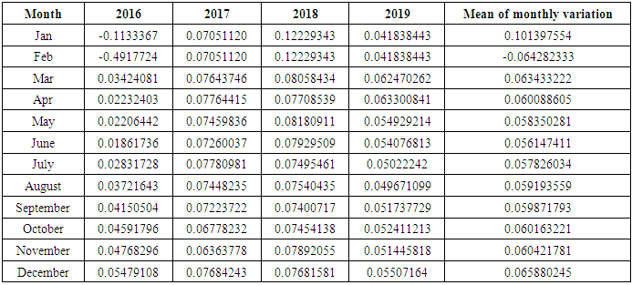
  But we us this relation Mean of monthly variationThis calculated for every month by the equation below
 | (3.3.1) |
 is not related to any other group.We will get Forecasted Value of the fuzzy membership by mid value
  (1+ average mean of monthly variation) (3.2.2).Fourth step: the difficult step and final step how many order equation I will use first, second, third order equation.In the method in section 3.2 use first order equation but in our Proposed Method twelve order equation but the condition here you must choose the data equal for example we choose data from January 2015 to December 2019 has 60 elements And we need prediction for 12 months so the data will be equal 60/12=5.
 4. Model Evaluation
- The process of evaluating models is intended to evaluate the field suitability of the model for the pattern in which the series data is running or the accuracy of the model in predicting the values of the current and future series, and there are many measures of the suitability of the model all depend on the degree of error, which is the difference between the actual value of the series at a specific time And the string value that the model expected at that time. In this study, we will rely on the following methods to compare the two models used in this paper to find out which one is more accurate in prediction.
4.1. Mean Absolute Percentage Error (MAPE)
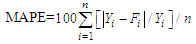 | (4.1.1) |
4.2. Mean Absolute Deviation (MAD)
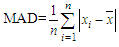 | (4.2.1) |
5. Data Collecting and Processing
- The data used in this research was gathered by the https://www.ceicdata.com/en from 2015-01 to 2019-12. It contained the data of production and consumption electricity in china. in a dataset.
6. Experimental Results and Discussion
6.1. Result Fuzzy Time Series Method and Discussion
- The first step: The dynamics of total production over May 2015-December 2020 years (input data for retrospective forecast) and variation in total production between every next and previous month. Variation for the current month is understood to be the difference between the sizes of production in current and previous months. For example, variation for Aug 2015 is equal = Aug 2015 – July 2015 then 3738.04336 - 3220.84444 = 517.19892. To define a universal set U, first of all, the smallest and greatest variation values must be found over the period [Dec 2015, Dec2019], later, to ensure the smoothness of boundaries of the interval, adequate values D1, D2 (positive figures are selected. After that, the universal set U can be defined as
 , where
  is the smallest variation (Jan 2019),
  is the greatest variation (Mar 2019),
  Thus, the universal set U will be as follows: U= {-6900, 1500}.The second step: The universal set U must be divided into several equal intervals. In our case, this set U is divided into seven equally- length intervals: u1= [-6900,-5700], u2= [-5700,-4500], u3= [-4500,-3300], u4= [-3300,-2100], u5= [-2100,-900], u6= [-900,300], u7= [300, 1500]. Basically we calculated the length of the interval U which is (1500)—(6900) =8400 and divided it by 7:8400/7=1200, then we built our small intervals: (example: u1= [[-6900,-5700]] which has 1200 as magnitude.If we take into account the fact that forecasting with fuzzy time series exhibits the least average error, it’s necessary to find the middle points of the intervals: um1=-6300, um2=-5100, um3=-3900, um4=-2700, um5=-1500, um6=-300, um7=900..The third step: Fuzzy sets are defined on the universal set U. In this case “ the variation in total production” is a linguistic variable that assumes the following linguistic values: A1=(very low level production electric (VLLPE)); A2=(low level production electric (LLPE)); A3=(changeless production electric (CPE)); A4= (moderate production electric (MPE)); A5=(normal-level production electric (NLPE)); A6= (high-level production electric (HLPE)); A7=(very high-level production electric (VHLPE)). To every linguistic value here corresponds a fuzzy variable which, according to a certain rule is assigned against a corresponding fuzzy set determining the meaning of this variable.For example, the linguistic value “very-low-level production electric” is given by the fuzzy variable <VLLPE, = [-6900,-5700], A1>, where A1 is a fuzzy set defined on the domain = [-6900,-5700] of the universal set U. See example (3).The fuzzy set A1, A2… A7 is defined on the universal set U by the following formula (6.1.1):
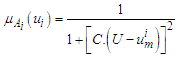 | (6.1.1) |
 is the middle point of the corresponding interval in (1); C is a constant. C is chosen in such a way that it ensures the conversion of definite quantitative values into fuzzy values or their belonging to the interval. (In our case C=0.0001);
 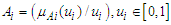 is a fuzzy setIf the value of the variable U in formula (6.1.1) is accepted as the middle point of the corresponding interval, the fuzzy set
  (i=1... 7) will be defined as follows:A1={(1/u1),(0.61/u2),(0.27/u3),(0.15/u4),(0.10/u5),(0.06/u6),(0.04/u7)}A2={(0,61/u1),(1/u2),(0.61/u3),(0.27/u4),(0.15/u5),(0.10/u6),(0.06/u7)}A3={(0,27/u1),(0.61/u2),(1/u3),(0.61/u4),(0.27/u5),(0.15/u6),(0.10/u7)}A4={(0,15/u1),(0.27/u2),(0.61/u3),(1/u4),(0.61/u5),(0.27/u6),(0.15/u7)}A5={(0,10/u1),(0.15/u2),(0.27/u3),(0.61/u4),(1/u5),(0.61/u6),(0.27/u7)}A6={(0,06/u1),(0.10/u2),(0.15/u3),(0.27/u4),(0.61/u5),(1/u6),(0.61/u7)}A7={(0,04/u1),(0.06/u2),(0.10/u3),(0.15/u4),(0.27/u5),(0.61/u6),(1/u7)}The fourth step: This step consists of the fuzzification of the variation calculated at the first step. This time, if
  is a variation for the i-th month, then membership function for
  is calculated by means of formula (6.1.1) by holding valid the equality
  that’s to say, by separating the interval, to which belongs the considered variation, from the universal set U. Here,
  is a fuzzy set of the corresponding variation for the year t= m×n where May2015<t Dec2019.The fifth step: We must select a basis w (1<w<l, where
  is the number of months, prior to the current month included in experimental evaluation). Resting on the basis W or the past months, we calculate a fuzzy relationship matrix
  by means of which is given a forecast. For this purpose, after the selection of w, we establish an operation matrix i×j
  (here i is the number of rows, Criteria matrix
  (a row matrix corresponding to fuzzy variation in total population for the month t-1). For example, by assuming that w=7, we can define the operation matrix
  (which is the matrix of fuzzy variations in total production electric over the months t-2, t-3, t-4, t-5, t-6, t-7) and the criteria matrix
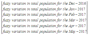
  (which is the fuzzy variation matrix for the month t-1). Thus for w=7, the previous 8 months data are utilized (the total production electric of the (t-8) month must be known to find variation of the (t-7) month).At last, for example, in order to forecast the total production electric for July 2017, the operation matrix О7 (т) will be established as follows
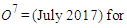
 О7 (1990) =
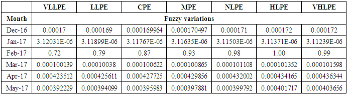 К (Jul-2017) = [fuzzy variation in total production electric for the Jun2017-th month] - [fuzzy variation in total population for Jun-2017], That is to say
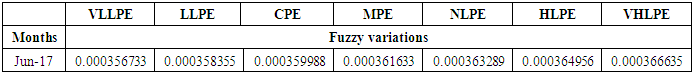 According to the method, the relationship matrix R (t) is calculated at the next step
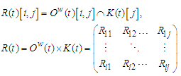 | (6.1.2) |
 is an operation matrix;
  is matrix of fuzzy sets,
  an operation min
  Later there is defined the forecasted value F (t) for the t year in a fuzzy form as follows.
 | (6.1.3) |
 Finally, the results obtained from population forecast for the July 2017 will be as follows.
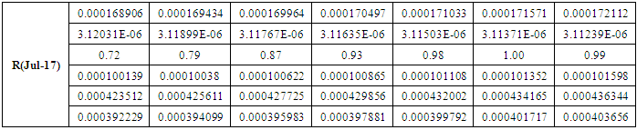
 Forecasting results for other years are calculated in an same manner.The sixth step: to fuzzify the obtained results of the 5-th step, the following formula is proposed
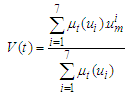 | (6.1.4) |
 is the calculated value of membership function for the forecast year t,
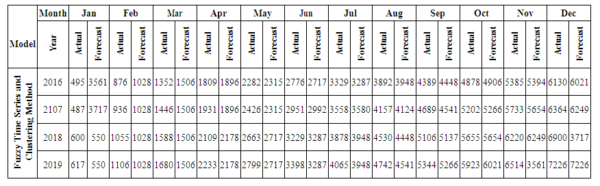
  are the middle points of intervals. For example, after calculating F (Jul-17) = -2.511164519, that is to say, anticipated production electric July 2017 equals to -2.511164519. In orders to estimate the forecasted total production electric for July 2017, we must add the calculated production electric to the total production for the June 2016. In other wordsN (July 2017) = 2959.83+-2.511164519=2957.32.Table 6.1.1 and Table 6.1.2 below show the actual and forecasted values of production and consumption electric for period from January 2016 to December 2019 in GWh the result has been rounded to the nearest integer.
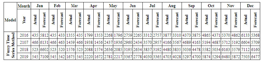 | Table 6.1.1. Actual and forecasted values of production electric in GWh |
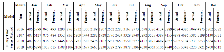 | Table 6.1.2. Actual and forecasted values of consumption electric in GWh |
6.2. Result Fuzzy Time Series and Clustering Method and Discussion
- The Proposed Method using the First Order Fuzzy Time Series.[Step 1] Apply the proposed clustering algorithm to partition UoD into different lengths of intervals.[Step 2] Sorting the numerical data: 5814.57, 435.09, 435.09, 1355.14, 1798.59, 2267.61, 2759.49, 3312.05, 3877.16, 4373.23, 4864.69, 5370.08, 6133.16, 465.77, 465.77, and 1458.72…..etc. Calculate the threshold
 for stopping condition of the proposed clustering algorithm:
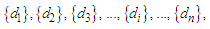
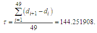 [Step 3] Put each datum in a cluster, shown as follows: {5814.57}, {435.09}, {435.09}, {1355.14}, {1798.59}, {2267.61}, {2759.49}, {3312.05}, {3877.16}, {4373.23}, {4864.69}, {5370.08}, {6133.16}, {465.77}, {465.77}, {1458.72}, {1938.24}, {2436.77}, {2959.83}, {3569.76}, {4165.94}, {4689.14}……………etc..[Step 4] Based on Eq. (2), calculate each cluster center
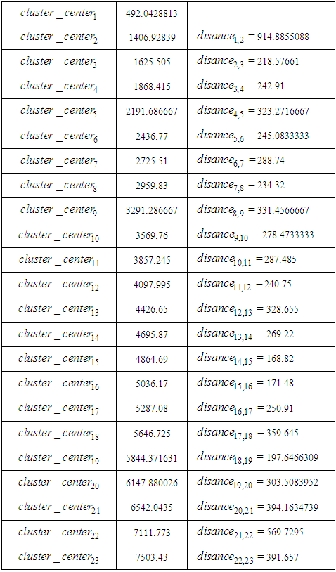
 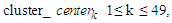 Based on Eq. (3.2.2), calculate the
 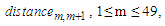 shown as follows: Find the smallest distance smallest_distance, i.e., 30.68 (the distance distance 2, 3 between
  Table 6.2.1 show the Distance between clusters for production electric
|
 i.e., 30.68 < 144.2519077 is true, then
  (i.e., {465.77}) and
  (i.e., {522.73}) are combined into one cluster (i.e., {465.77, 522.73}), and go to Step 2 the iterations of Step 3 to Step 5 are repeatedly done until the condition
 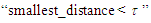 is false.
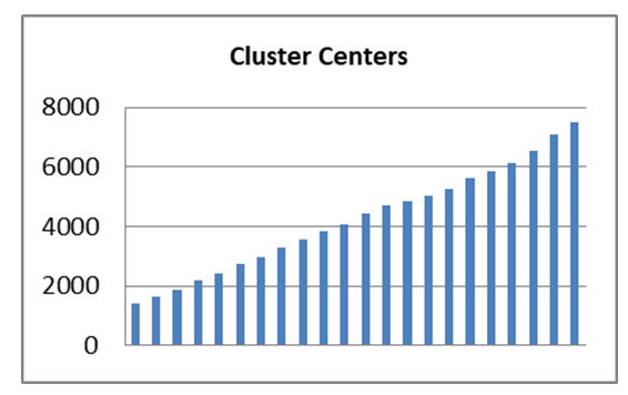 | Figure 1. Cluster centers of production electric |
 Because there is no previous cluster before
  , the lower bound of
  of
of  is calculated using Eq. (3.2.4) and because there is no next cluster after the last cluster, i.e.,
  the upper bound
  is calculated using.
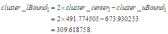
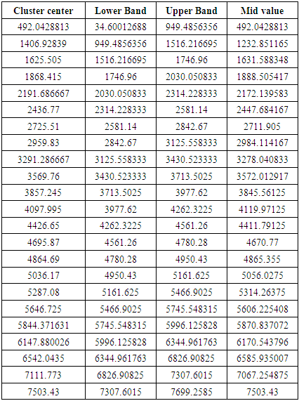
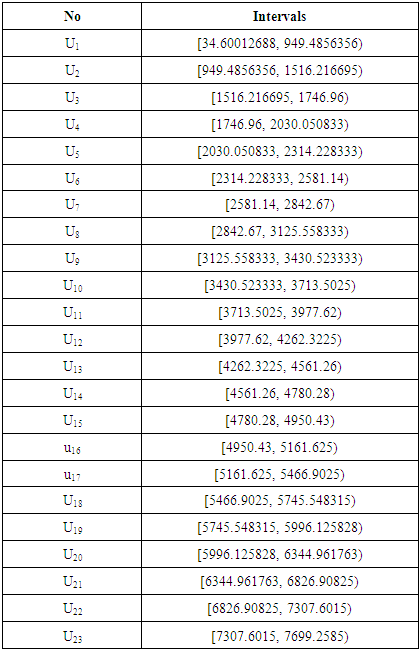
 [Step 7] Let each
  form an
  and calculate the middle value using Eq. (3.2.5). The table 6.2.2 below shows Interval Generations from the Clusters and Final intervals from clusters show in table 6.2.3.
|
|
 ,shown as follows:
 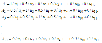 [Step 2] Fuzzify each datum that is belonging to ui, where 1≤ i ≤ 11 into Ai.[Step 3] Obtain the fuzzy logical relationships (FLR) of the first order fuzzy time series Table (6.2.4). Let the FLR having the same current state to form a FLR group (FLRG).
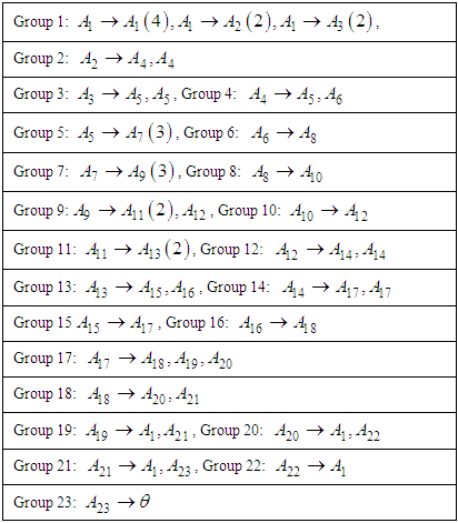
|
|
 | Table 6.2.6. Actual and forecasted values of production electric in GWh |
 | Table 6.2.7. Actual and forecasted values of consumption electric in GWh |
6.3. Result Proposed Method for Predicting Using Fuzzy Time Series and Clustering Discussion
- The Proposed Method using Fuzzy Time Series and Clustering the same steps but we will use data from January 2015 to December 2019 in our proposal method we will us we use time-invariant fuzzy time series in section 3.1, the first step and second step The same in section 4.2 and will start from step three in proposed method.[Step 3] Obtain the fuzzy logical relationships (FLR) of the first order fuzzy time series. Let the FLR having the same current state to form a FLR group (FLRG).In Figure 2, this histogram gives us a clear idea about the distribution of our data, we can see that
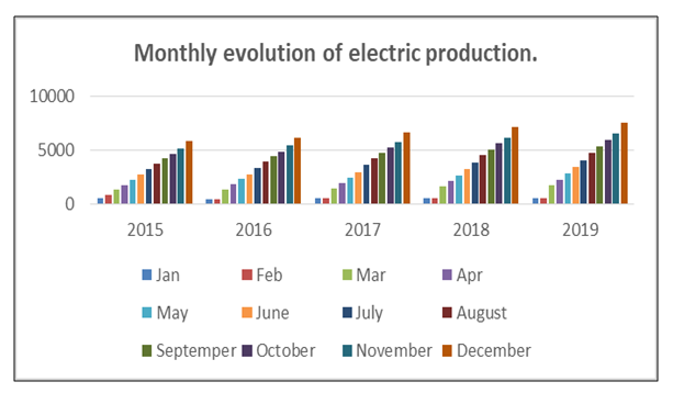 | Figure 2. Monthly evolution of electric production |
 .
.
|
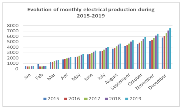 | Figure 3. Monthly evolution of electric production |
|
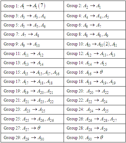
 which state come after state A26the forecasted value of A27 by equation (3.2.2)Mid value (1+ average mean of monthly variation)
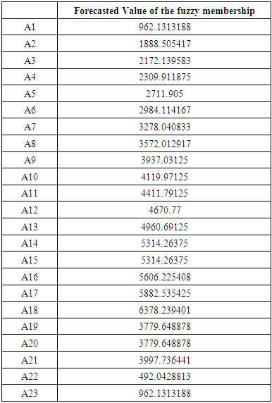
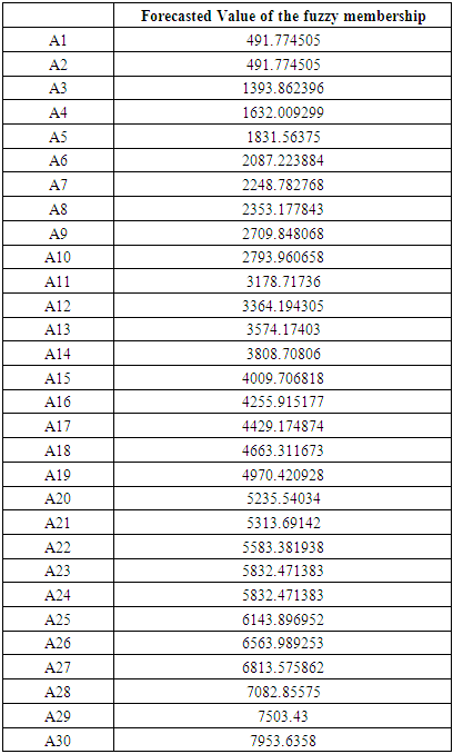
 [Step 5] Calculate the forecasting value. In column 1 from table 6.3.3 we start forecasting our data by using states from the previous year. How we do this? Let's see some examples: We forecast the value of February 2016 by looking at the state of February 2015 and we affect the corresponding forecasted value from column C which is (491, 774505).We forecast the value of July 2016 by looking at the state of July 2015 and we affect the corresponding forecasted value from column C which is (3364, 194305). Table 6.3.4 and 6.3.5 below shows the actual and forecasted values of production and consumption electric for period from January 2016 to December 2019 in GWh, the result has been rounded to the nearest integer.
|
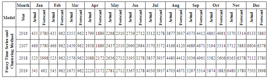
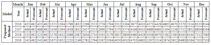 | Table 6.3.4. Actual and forecasted values of production electric in GWh |
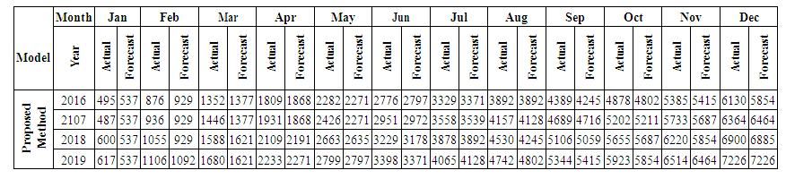 | Table 6.3.5. Actual and forecasted values of consumption electric in GWh |
7. Conclusions
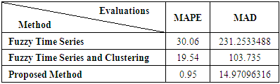
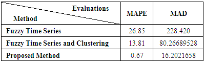
- The forecasts obtained utilizing Fuzzy time series method and Fuzzy Time Series and Clustering and Proposed Method are discussed in this paper. The aforementioned methods require only the historical data series of electricity consumption to build the forecast. This can be considered as an important advantage, because the effort and cost linked to the data mining are very limited. These historical time series data are analyzed to understand the past and predict the future. Mean Absolute Percentage Error the mean absolute deviation.The results of predictive metrics of electricity production indicated that the Mean Absolute Percentage Error ranged from 0.95 (Proposed Method) to 30.06 Fuzzy Time Series method and mean absolute deviation ranged from 14.97096316 (Proposed Method) to 231.2533488 Fuzzy Time Series method, Fuzzy Time Series and Clustering method performed closed to the Proposed Method but Fuzzy Time Series method deviated a lot (Table 7.1), (Table 7.2). So, this criterion clearly indicated the superiority of Proposed Method in forecasting the production of electricity and consumption electric during 2016-2019. Similarly, the Proposed Method gave the lowest value thus performed best followed more than Fuzzy Time Series and Fuzzy Time Series and Clustering methods. Fuzzy Time Series method performed the worst in all cases. Similar to the prediction of electric energy production, Proposed Method performed best when the consumption of electric energy was predicted. But it is quite interesting that in case of forecasting the electric energy consumption.
|
|
|
|
 | Figure 4. Balance in Energy Production and Consumption for Electric |