Azeez M. B. , Olanrewaju S. O.
Department of Statistics, Faculty of Science, University of Abuja, Abuja, Nigeria
Correspondence to: Olanrewaju S. O. , Department of Statistics, Faculty of Science, University of Abuja, Abuja, Nigeria.
| Email: |  |
Copyright © 2020 The Author(s). Published by Scientific & Academic Publishing.
This work is licensed under the Creative Commons Attribution International License (CC BY).
http://creativecommons.org/licenses/by/4.0/

Abstract
This study empirically examined the impact of macroeconomic variables (exchange rate, gross domestic product, inflation and interest rate) on stock market prices in Nigeria using quarterly time series data covering the period 1989; 1 to 2018; 3. The econometric technique employed in the research is the Generalized Autoregressive Conditional Heteroscedasticity (GARCH) model. The econometric analysis began with pre-diagnostic test which is a pre-condition for estimating GARCH model (testing for clustering volatility and ARCH effect in the residual). Properties of the time series variables were examined and tested for stationarity using the Augmented Dickey-Fuller (ADF) unit root test. The test revealed that all the variables; all share index, exchange rate, gross domestic product, inflation and interest rate were stationary at either level I(0) or at first difference I(I). The conditional variance equation of the GARCH model revealed that GDP has positive effect on stock prices while other macroeconomic variables have negative effect on stock return volatility. The study found that stock prices is more responsive to their lag values than the variables of exchange rates, gross domestic product, inflation and Interest rate; and therefore, the study recommends the following: That Government should always embark on policies that will lead to substantial growth in the real gross domestic product; ensure that a decrease in interest rate is also accompanied by an increase in investment. Thus, interest rate should be guided by the relevant authority through a preferred range for investing firms; and finally ensure a relatively stable exchange rate and keep Inflationary trend at a single digit.
Keywords:
Microeconomic variables, GDP, ARCH, GARCH
Cite this paper: Azeez M. B. , Olanrewaju S. O. , Statistical Analysis on the Impact of Macroeconomic Variables on Stock Market Prices in Nigeria, International Journal of Statistics and Applications, Vol. 10 No. 2, 2020, pp. 34-42. doi: 10.5923/j.statistics.20201002.02.
1. Introduction
Over the past few decades (1980-2010), the connection between macroeconomic variables and the movement of stock market prices has been a subject of interest among academics and researchers [1]; [2]. It is often argued that stock prices are determined by some fundamental macroeconomic variables such as interest rate, exchange rate, gross domestic product, inflation, oil prices and money supply.[3] identifies gross domestic product (GDP), inflation rates, interest rates, exchange rates, government fiscal position, infrastructure and political factors to be the macroeconomic fundamentals that could exert shocks on stock prices and influence investors’ investment decisions. This is because the changes in stock prices and the trend of changes have always been of interest in the capital market stability and strategies adopted by investors [4].However, a well-organized stock market makes an attractive feature of issuing and investing in stocks. From the corporation’s perspective, the stock market allows it to raise funds by selling additional shares of ownership. On the other hand, it also provides liquidity to investors (investors are able to quickly and easily convert their securities to cash). It is an institution where the securities of joint stock companies are traded freely and the prices are determined by the forces of supply and demand. Simply put, it is a place where buyers and sellers come together to exchange their holdings (shares, bonds, derivatives etc.) during business hours.The Nigerian stock market (NSE) has seen drastic volatility in its performance such that for example between March 2007 and July 2011, the NSE market capitalization has recorded a variation from a high of 12.6 trillion naira to a low of 7.6 trillion naira with All- share index from 66,371 points to 23,826 points.
1.1. Aim and Objectives of the Study
Given that economic activities in Nigeria have been changing and that macro-economic variables have taken different values over the years alongside stock prices, the main objective of this study, therefore, is to examine the impact of some key macro-economic variables such as gross domestic products, exchange rates, interest rates and inflation rates volatility on stock prices and to determine the magnitude and direction of their influence on stock prices in Nigeria.Hence, the specific objectives of this study are:(i) Examine the trends in the movements of the macroeconomic variables and stock prices in Nigeria.(ii) To estimate if a long run relationship exists between the macroeconomic variables and the stock market prices in Nigeria.To determine whether gross domestic product, exchange rates, inflation rates and interest rates significantly affect the volatility of stock market prices in Nigeria.
2. Review of Some Relevant Literature
2.1. Conceptual Literature Review
Stock market can be defined as an institution where the securities of joint stock companies are traded freely and the prices are determined by the forces of supply and demand. Simply put, it is a place where buyers and sellers come together to exchange their holdings (shares, bonds, derivatives etc.) during business hours. It is the citadel of capital, the temple of values and the axe of which the whole financial structure of the capitalist system turns [5]. Furthermore, [6] the stock exchange can also be a mechanism (barometer as some would suggest) which can measure and detect the systems of an impending economic boom or decline long before the predicted prosperity or decline actually occurs. All over the world, stock markets act as important catalyst for economic growth and development. Without a fully developed stock market, a country would not be able to grow its equity funding and move towards more balanced financial structures as the stock exchange is the engine room for fund generation as the market enables publicly traded companies to raise investment capital through the sale of shares to investors.Stock market reacts in response to various factors ranging from economic, political and socio-cultural behavior of any country. It supports resource allocation and spurs growth through different channels. By reducing transaction costs and liquidity costs, stock markets can positively affect the average productivity of capital. By pooling resources for larger projects which would otherwise have difficulty accessing finance, stock markets can mobilize savings and spur the rate of investment. Through the promotion of acquisition of information about firms, stock markets may promote and improve resource allocation and the average productivity of capital.
2.2. Empirical Literature Review
Many researchers, financial analysts and practitioners have attempted to predict the relationship between stock market movement and macroeconomic variables. They have conducted empirical studies to examine the effect of stock price on macroeconomic variables or vice-versa. This section of the paper has discussed some such previous research works and their empirical conclusions that are related to our sector analysis.[7] conducted a study on the relationship between stock prices and exchange rate in four South Asian countries; Pakistan, India, Bangladesh and Sri-Lanka for the period 1994 to 2000. The study employed co-integration, vector error correction modeling techniques and standard Granger causality tests to examine the long run and short run association between stock prices and exchange rates. The result of the study showed no short run association between the variables for all the four countries. There was no long run relationship between stock prices and exchange rates for Pakistan and India as well. [8] investigated the effects of exchange rate volatility on the stock market in South Africa, using GARCH model for the period 2000 to 2010. The study used market capitalization as proxy to stock market prices. The result found very weak relationship between currency volatility and the stock market.[9] empirically investigates the relationship between macroeconomic variables and stock returns under the Arbitrage pricing theory framework from the period 2005 to 2010. Ordinary Least Square method was applied and findings reveal that a significant variation in stock market return is caused by consumer price index, short term interest rate and money supply. [10] investigate the causal relationship between stock prices and exchange rate, using data from 23rd February 2001 to 11th January 2008 about turkey. The reason for using this period is that exchange rate regime is determined as floating in this period. The result of empirical study indicates that there is bi-directional causal relationship between exchange rate and all stock market indices. [11] evaluates the effect of exchange rate volatility on stock prices in Nigeria over the period 1985 to 2014 with a view to ascertain the extent of currency volatility on stock prices as well as its stability in reducing volatility in Nigeria stock exchange market, using real exchange rate, interest rate, money supply and inflation. The Garch model was employed. His result revealed that real exchange rate and inflation rate has more effect on stock prices, while money supply has a positive effect on stock prices and interest rate has a negative effect.Result from GARCH-X model shows that NSE return volatility is positively influenced by changes in broad money supply and inflation rate. Net foreign asset shows a negative but significant influence in stock returns.
3. Research Methodology
3.1. Generalized Autoregressive Conditional Heteroscedasticity (GARCH) Breakdown
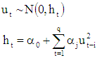
In Econometrics the autoregressive conditional heteroscedasticity (ARCH) model is a statistical model for time series data that describes the variance of the current error term or innovation as a function of the actual sizes of the previous time periods' error terms; often the variance is related to the squares of the previous innovations. The ARCH model is appropriate when the error variance in a time series follows an autoregressive (AR) model; if an autoregressive moving average (ARMA) model is assumed for the error variance, the model is a generalized autoregressive conditional heteroskedasticity (GARCH) model.ARCH models are commonly employed in modeling financial time series that exhibit time-varying volatility and volatility clustering, i.e. periods of swings interspersed with periods of relative calm. ARCH-type models are sometimes considered to be in the family of stochastic volatility models, although this is strictly incorrect since at time t the volatility is completely pre-determined (deterministic) given previous values.There are basically three different types of GARCH models which are GARCH, GJR-GARCH and EGARCH model. ARCH Model ARCH models based on the variance of the error term at time t depends on the realized values of the squared error terms in previous time periods. The model is specified as: | (1) |
 | (2) |
This model is referred to as ARCH(q), where q refers to the order of the lagged squared returns included in the model. If we use ARCH (1) model it becomes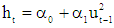 | (3) |
Since  is a conditional variance, its value must always be strictly positive; a negative variance at any point in time would be meaningless. To have positive conditional variance estimates, all of the coefficients in the conditional variance are usually required to be non-negative. Thus, coefficients must be satisfied
  and
and  .GARCH ModelThe model allows the conditional variance of variable to be dependent upon previous lags; first lag of the squared residual from the mean equation and present news about the volatility from the previous period which is as follows:
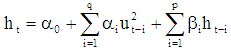 | (4) |
In the literature most used and simple model is the GARCH (1,1) process, for which the conditional variance can be written as follows: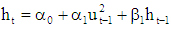 | (5) |
Under the hypothesis of covariance stationarity, the unconditional variance  can be found by taking the unconditional expectation of equation 5.We find that
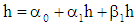 | (6) |
Solving the equation 5 we have 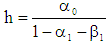 | (7) |
For this unconditional variance to exist, it must be the case that  and for it to be positive, we require that
  .GJR GARCHThe GJR model is a simple extension of GARCH with an additional term added to account for possible asymmetries. This GARCH model which allows the conditional variance has a different response to past negative and positive innovations.
 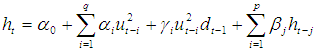 | (8) |
where  is a dummy variable that is:
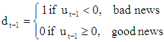 In the model, effect of good news shows their impact by
  , while bad news shows their impact by
  . In addition, if
  news impact is asymmetric and
  leverage effect exists. To satisfy non-negativity condition coefficients would be
  ,
,  ,
,  and
and  . That is the model is still acceptable, even if
  , provided that
  .Exponential GARCH Exponential GARCH (EGARCH) proposed by Nelson (1991) which has form of leverage effects in its equation. In the EGARCH model the specification for the conditional covariance is given by the following form:
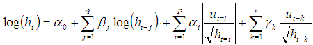 | (9) |
Two advantages stated for the pure GARCH specification; by using  even if the parameters are negative, will be positive and asymmetries are allowed for under the EGARCH formulation.In the equation
  represent leverage effects which accounts for the asymmetry of the model. While the basic GARCH model requires the restrictions the EGARCH model allows unrestricted estimation of the variance. If
  it indicates leverage effect exist and if
  impact is asymmetric. The meaning of leverage effect bad news increase volatility.Applying process of GARCH models to return series, it is often found that GARCH residuals still tend to be heavy tailed. To accommodate this, rather than to use normal distribution the Student’s t and GED distribution used to employ ARCH/GARCH type models.
3.2. Sources and Methods of Data Collection
Nigerian Stock Exchange (NSE) All Share Index (ASI) was used to measure the stock market trends and performance. The sample period spans from 1986 to 2016, consisting of 123 quarterly data for each variable. The possibility of getting quarterly data before 1986 compelled the researcher to choose 1986 as the starting year and also because it marks the year Nigerian government embarked on Structural Adjustment Programme (SAP) which made Nigerian Stock Market became more accessible to the international community around this period. This is an important consideration since the exchange rate is one of the four macroeconomic variables. This will enable the investigation of the extent to which the economy has achieved the cardinal objective of exchange rate stability. The time series data set was sourced from various issues of the Central Bank of Nigeria Statistical Bulletin and Bullion, Security and Exchange Commission and NSE fact book and annual reports.The data series were subjected to the appropriate time series tests using EVIEWS 9 econometric software which is time series friendly.
4. Data Analyses and Results Discussions
4.1. Introduction
The Johansen co-integration test, and the results of the Generalized Autoregressive Conditional Heteroskedasticity (GARCH) model (1,1) the section further provide the pre- and post-estimation diagnostic tests. In the last section, discussion of the results in relation to those reviewed in the literature and the policy implications of findings are presented.
4.2. Descriptive Statistics for Quarterly Data on Stock Prices (All Share Index)
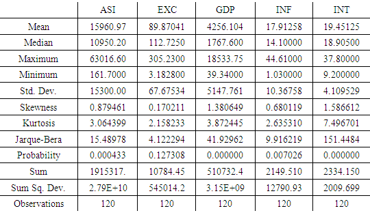
Table 4.1 below contains basic descriptive statistics for quarterly stock returns of the Nigeria’s stock market. Table 4.1. Descriptive statistic for ASI, exchange rate, GDP, inflation and interest rate
 |
| |
|
The summary of the data used in estimating the impact of macroeconomic variables on stock market prices in Nigeria from 1989 to 2018 are presented in Table 4.1. We examined 123 observations for each of the variables to estimate the descriptive statistics. The mean describes the average value in the series. Standard deviation measures the volatility of the data or the amount of deviation or dispersion of the data from the average. The skewness measures whether the distribution of the data is symmetrical or asymmetrical. A positive skewness value indicates that the distribution of the data has a long right tail, while a negative skewness value shows that the distribution of the data has a long-left tail. Kurtosis measures the peakedness of the data compared to normal (leptokurtic).However, the table shows that all the macroeconomic variables have positive mean return values, the average all share index (ASI), exchange rate, GDP, inflation rate and interest rate are 8.686219, 3.869542, 7.185864, 2.684993, and 2.930714 values points respectively for the 123 Observations, which is relatively normal. The standard deviation of all share index, exchange rates, GDP, inflation and interest rate are 1.818510, 1.358425, 1.861496, 0.675593 and 0.223190 respectively. They are much lower than their mean values, thereby indicating that their prices have been expressly unstable over the years. This result is confirmed by the negative skewness values (showing that all the macroeconomic variables values in the sample are lesser than the mean value) and the P-values associated with the Jarque-Bera statistics, a test for departure from normality, show that all the variables under study deviates normal distribution. The non-normality of the variables is supported by their skewness and kurtosis coefficients. The kurtosis and skewness of a normally distributed series are three and zero respectively. Thus, all share index, exchange rate and GDP all have values below three (3) which implies a platykurtic kurtosis, while inflation and interest rate has value higher than three (3) and this indicate a leptokurtic.
4.2.1. Unit Root Test Results
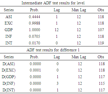
As a precondition for the analysis of time series variables, the need to ensure that the variables are stationary requires unit root tests of each of the variables in the model. The outcome of our unit root tests using the Augmented Dickey Fuller (ADF) test revealed that all the variables are stationary, some at level I(0), and some at first difference I(1). The results are presented in the Table 4.2. Unit Root Tests Results
 |
| |
|
As a first step in the analysis, unit roots test was conducted to know the stationarity properties so as to avoid spurious regression. The result revealed that all the variables were stationary at levels at 10% only, except GDP. Given their probability values that is greater than 5%, and this necessitates testing at first difference. With the first difference level of the variables, the result revealed that, all the variables were stationary at first difference which means that they were all integrated of order one {I(1)}.
4.2.2. Johansen Co-integration Test Results
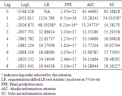
Table 4.3. Selection of lag length for co-integration test
 |
| |
|
To test for co-integration, it is important to determine the appropriate lag length. Table 4.3 present the results of the optimal length of lag selection for the co-integration, based on the five information criteria. The Schwarz (SC) and Hannan-Quinin (HQ) information criterion, which are most widely used, suggested that a lag length of one is optimal for the test. Therefore, this study used a lag length of one for the test of co-integration ranks and for the subsequent diagnostics test for data analysis.Table 4.4. Johansen Co-integration Test Results
 |
| |
|
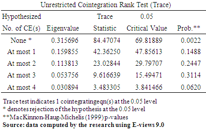
A test for co integration is a test to avoid spurious regression situation but based on the result of the co integration test, we do not accept the null hypothesis because there is existence of a long run relationship among variables. It reveals that there is existence of one co-integrating equation in the system with its maximum Eigen value and trace statistics greater than the critical values at 5 per cent. Therefore, the null hypothesis of no co-integration is rejected in favor of the alternative hypothesis of the presence of co-integration among the variables. Based on the result, we concluded that a long run relationship is present among the actual variables as shown by the Max- Eigen value and the trace statistics (none*), as both values are higher than the 5% value as presented in the above table.
4.3. Pre-Diagnostic Tests for GARCH Model
As a precondition for estimation of GARCH model, a test for its suitability in the analysis was conducted by estimating whether there is clustering volatility in the residual, and testing for the ARCH effect.
4.3.1. Test for Clustering Volatility
Clustering volatility means when the periods of low volatility are followed by periods of low volatility, and periods of high volatility are followed by periods of high volatility for a prolonged period. This is shown in the table below: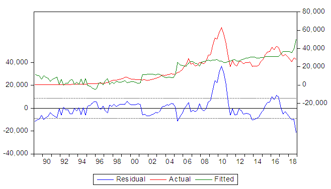 From the above table, the periods between 1989 and 2003 shows a prolong periods of low volatility followed by periods of low volatility. While the periods between 2004 and 2018 indicates that periods of high volatility are followed by periods of high volatility. It suggests that the residuals or error term is conditionally heteroscedastic and it can be represented by ARCH and GARCH model.
4.3.2. Test for ARCH Effect
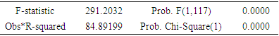
The second pre-test for the application of GARCH model is the ARCH effect. Here, the study tests the null hypothesis (H0) that there is no ARCH effect against the alternative hypothesis that there is ARCH effect (H1). This test is presented inTable 4.5. Heteroskedasticity (ARCH Effect) Test
 |
| |
|
From Table 4.5 above, the chi-square probability is less than 5% which shows that there is ARCH effect. From the foregoing, there is clustering volatility in the residual and ARCH effect which implies that chosen GARCH (1.1) model is suitable for the analysis. The study therefore, proceeded to estimate the GARCH model as follows. The foregoing result on clustering volatility and ARCH effect is in conformity with the works of [8].
4.4. Estimated Results of the Mean Equation
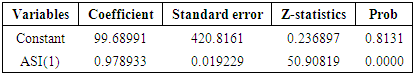
The estimated results of the mean equation are presented in Table 4.6.Table 4.6. Results of the Mean Equation
 |
| |
|
The mean equation as presented in Table 4.6 above reveals that the impact of lagged stock prices is significant at 5% level of significance. This implies that previous quarter value of stock prices can influence the current quarter values of the variable. The coefficient is 0.978933. This implies that there seems to be a very long delay for share prices to return to its long run position after any shock. Thus, stock price shocks are seen to be persistent over time.
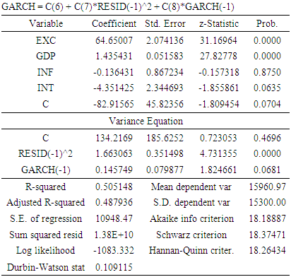
4.5. Results of the Conditional Variance Equation in the GARCH (1.1) Model
The estimated results of the conditional variance equation in the GARCH (1.1) model are presented in Table 4.7 below. Table 4.7. Results of the Conditional Variance Equation in the GARCH (1.1) Model
 |
| |
|
The equation of interest in the GARCH (1.1) model is that of the conditional variance equation which measures the effects of the macroeconomic variables on stock price volatility. The results are shown in Table 4.7. They reveal that the ARCH term (δ2t-1) coefficient is 0.915777 and its P-value is 0.0000 which is less than 5%. This implies that previous quarters of all share index (ASI) information can exert or influence the volatility of present quarter of ASI in Nigeria. While the GARCH term (ht-1) coefficient is 0.54182 and its P-value 0.0000 is less than 5% which also indicates that the past quarters volatility of ASI can affect present quarter volatility of ASI. A large positive value of ARCH (α1) shows that strong volatility clustering is present in the time series in question. And a large value of GARCH (α2) reveals that the impact of the shocks to the conditional variance lasts for a long time before dying out, so volatility is persistent following a crisis in the Nigerian market. Thus, long term measures must be put in place when taking short term arbitrary stock prices shocks in the Nigerian stock market. The positive value of the GARCH effect or GARCH coefficient also shows the tendency of stock prices gaining upward slide at any given shock. This GARCH effect is significant at 5%. The conditional variance results also suggest that changes in US dollar/Naira exchange rates has negative effect on stock price. It reveals that a percentage increase in exchange rate results in 134% reduction in stock return, and this is statistically significant at 10% level because its probability value (09.96%) is less than 10%. The result on GDP shows that it has positive impact and not statistically significant on stock price volatility, because its probability value is 20.19%. Inflation rates coefficient is -1.576149 and it has negative impact on stock returns volatility but significant at 5%. While the last macroeconomic variable examined in the study (interest rate) also have negative effect or impact on stock price return volatility (-5.050980), and the results are statistically significant at 5%. The estimated results of the conditional variance equation for each of the macroeconomic variables in the GARCH (1,1) model are all in line with the a-priori expectations of the study. The diagnostic statistics of the results reveal that the adjusted R squared value is 0.022958 which means that only 2.2 percent of the systematic variations or volatility in stock prices is determined by the explanatory variables in the variance equation. This implies that there are more macroeconomic variables outside the model that significantly affect the stock price volatility. The Durbin-Watson (D-W) statistic is 1.430115 this means that there is absence of autocorrelation in the residuals of the model over time as the D-W statistic is close to two.
4.6. Discussion of Findings
This research work has empirically examined the impact of macroeconomic variables (exchange rate, GDP, inflation and interest rate) on stock prices in Nigeria using quarterly time series data analysis ranging from 1989: 1 to 2018: 3. Firstly, ADF test was carried out in testing for the stationarity of the variables, and the outcome of our unit root tests revealed a mixture of integration order, I(0) and I(1) among our variables. The discussion of the outcome examines how the results of this research, earlier explained are in line with or different from similar studies previously conducted.To start with, the result on exchange rate revealed that it has negative relationship but statistically significant on stock price volatility. So, we therefore, reject H01 that exchange rate has no significant impact on stock prices in Nigeria. This is in line with the findings of [12]. On the relationship between GDP and stock prices, the study revealed that it has positive impact but has no statistically significant effect on stock prices. This evidence of positive effect of GDP on stock prices is consistent with the findings of [13] which revealed positive and long run relationship with stock prices in Nigeria.For the third independent variable (inflation rate), the hypothesis H01 postulated that; increasing rate of inflation has no significant impact on stock prices in Nigeria. While the result indicated that ASI return volatility is negatively influenced by changes in inflation rate and thus, the null hypothesis is rejected. This aligns with the findings of [14].The findings of interest rate deviate from that of [15], who examine the relationships between stock returns and interest rates from 1984 to 2007. They find that prevailing interest rates, exerts positive influence on stock prices. While the result on interest rate revealed negative relationship but shows statistically significant effect on stock price volatility. So, we reject H01 and accept alternate hypothesis that there is a negative significant relationship between interest rate and stock prices in Nigeria and this finding is consistent with the works of [16]. The interest rate result depicted a high interest rate in Nigeria. Monetary policy decision made by the monetary authorities in their attempt to stabilize the economy is usually responsible for this. It could make access to credit difficult and thus make shares price less attractive.
5. Summary, Conclusions and Recommendations
5.1. Summary of Findings
The study has investigated the impact of macroeconomic variables on stock market returns in Nigeria. Some key macroeconomic determinants of stock price volatility in the Nigerian stock market were empirically examined. Since volatility was the goal of the study, the Generalized Autoregressive Conditional Heteroskedasticity (GARCH) model was employed in the empirical analysis. In view of the above, time series (Quarterly) data used covers the period 1989 to 2018 and were sourced from the CBN and NBS. The study did an explicit exposition on relevant literature to the study and also a theoretical framework to form the basis for the analysis. The main findings of the study are:• That stock prices in Nigeria are volatile in nature; rising and falling rapidly in successions. The GARCH model indicated a significant ARCH term in the analysis, suggesting that news or information in the market causes fluctuation in the prices.• That previous quarter volatility of all share index in the market also has a great effect and influence on present quarter stock price volatility in Nigeria. The GARCH term was also significant.• That interest rate is the main determinant of stock price volatility in Nigeria. Increase/decrease in leading rates tends to cause stock prices less or more attractively in the market.• That exchange rate, inflation rate and interest rate have negative relationship on stock price volatility in Nigeria.
5.2. Conclusions
It has become obvious that the factors behind changes in stock prices may be potent enough to create necessary directions in overall stock market performance in Nigeria. In this study, it has been shown that only interest rate, among the monetary and real sector variables, exerts pressure on the stock prices in Nigeria. The analyses demonstrate that the Nigerian stock market is actually an emerging one where a strong competition is beginning to develop between the stock market and the other financial sector in terms of their instruments.However, this pace of development should be handled with care because any false movements in the stock market may have resounding impact in the whole financial sector and even the entire economy. Findings of this paper suggest that the government should be cautious with how interest rates and inflation rate are managed since they have ramifications for the budding stock price. In the years to come, it is likely that Central banks will be required to include financial stability among their macroeconomic responsibilities more directly and explicitly.
References
| [1] | Amado, C., & Teräsvirta, T. (2014). Conditional correlation models of autoregressive conditional heteroscedasticity with nonstationary GARCH equations. Journal of Business & Economic Statistics, 32(1), 69–87. |
| [2] | Audrino, F., & Bühlmann, P. (2001). Tree‐structured generalized autoregressive conditional heteroscedastic models. Journal of the Royal Statistical Society: Series B (Statistical Methodology), 63(4), 727–744. |
| [3] | Bond, S. A. (2001). A review of asymmetric conditional density functions in autoregressive conditional heteroscedasticity models. In Return distributions in finance (pp. 21–46). Elsevier. Central Bank of Nigeria Statistical Bulletin for Several Issues: http://www.cenbank.org/. |
| [4] | Chang, B. R. (2006). Applying nonlinear generalized autoregressive conditional heteroscedasticity to compensate ANFIS outputs tuned by adaptive support vector regression. Fuzzy Sets and Systems, 157(13), 1832–1850. |
| [5] | Francq, C., & Zakoïan, J. (2012). Strict stationarity testing and estimation of explosive and stationary generalized autoregressive conditional heteroscedasticity models. Econometrica, 80(2), 821–861. |
| [6] | Ilbeigi, M., Castro-Lacouture, D., & Joukar, A. (2017). Generalized autoregressive conditional heteroscedasticity model to quantify and forecast uncertainty in the price of asphalt cement. Journal of Management in Engineering, 33(5), 4017026. |
| [7] | Zhang, X., & King, M. L. (2005). Influence diagnostics in generalized autoregressive conditional heteroscedasticity processes. Journal of Business & Economic Statistics, 23(1), 118–129. |
| [8] | Courage Mlambo, Andrew M. and Kin S (2013), Effects of exchange rates volatility on stock market: a case study of South Africa. Mediterranean journal of social sciences, MCSER Publisher, Rome Italy. November 2013 |
| [9] | Sally, & Salihu A., (2011). Nigerian stock returns and macroeconomic variables: evidence from the APT, MBA, Eastern Mediterranean University, Gazimagusa, North Cyprus. |
| [10] | Daferighe, E.E. & Aje, S.O. (2009). An Impact Analysis of Real Gross Domestic Product, Inflation Impact and interest Rates on stock prices of Quoted Companies in Nigeria International Research Journals of Finance and Economics. |
| [11] | Aue, A., Horváth, L., & F. Pellatt, D. (2017). Functional generalized autoregressive conditional heteroskedasticity. Journal of Time Series Analysis, 38(1), 3–21. |
| [12] | Levine, R. (1997). Financial Development and Economic Growth: Views and Agenda. Journal of Economic Literature 35: 688-726. |
| [13] | Philip Ifeakachukwu NWOSA, Isiaq Olasunkanmi OSENI (2011). Efficient Market Hypothesis and Nigerian Stock Market. Research Journal of Finance and Accounting. Vol.2 No.12. Pp38-46. |
| [14] | Maku, O. E. and Atanda A. A., (2009). Does Macroeconomic Indicators Exert shock on the Nigerian Capital Market? |
| [15] | Ologunde, A. O., Elumilade, D. O. and Asaolu, T. O. (2006). Stock Market Capitalization and Interest Rate in Nigeria: A Time Series Analysis. International Research Journal of Finance and Economics, Issue 4. |
| [16] | Nwokoma, N.I., (2002). Stock Market Performance and Macroeconomic Indicators Nexus in Nigeria. An Empirical Investigation. Nigerian Journal of Economic and Social Studies, 44-2. |

 Abstract
 Reference
 Full-Text PDF
 Full-text HTML