Igbasan S. S., Olanrewaju S. O.
Department of Statistics, Faculty of Science, University of Abuja, Abuja, FCT, Nigeria
Correspondence to: Olanrewaju S. O., Department of Statistics, Faculty of Science, University of Abuja, Abuja, FCT, Nigeria.
| Email: |  |
Copyright © 2020 The Author(s). Published by Scientific & Academic Publishing.
This work is licensed under the Creative Commons Attribution International License (CC BY).
http://creativecommons.org/licenses/by/4.0/

Abstract
This study compares the forecasting models of Nigeria monthly Treasury Bill Data. The analysis is based on using monthly issues bill data from January 2011 to December 2018. Treasury bill rate of two short term Treasury bills (91 day and 182 day) from the year 2011 to 2018. The data were stationary at first difference but not normally distributed. ARMA, ARIMA and SARIMA models were computed and diagnosed. From the results of parameter estimation of the models, ARMA (2, 1) model was the best model among the other ARMA models computed using information criteria, (AIC). Diagnostic test was run on the ARMA (2, 1) model where the results showed that the model was adequate and normally distributed using Box-Ljung test and Q–Q plot respectively. Furthermore, ARIMA of first and second differences were estimated and ARIMA (2, 1, 1) was the best model from the result of the AIC and diagnostic test that were run and the model was found to be adequate and normally distributed from Box- Ljung and Q-Q plot respectively than ARIMA (2, 2, 1). From the results obtained in the ARMA and ARIMA model, ARIMA (2, 1, 1) x SARIMA (2, 1, 1)12 was now estimated and found to be adequate from the result of the Box-Ljung and Q-Q plot respectively. Post forecasting estimation and performance evolution was evaluated using the RMSE and MAE. The results showed that, ARIMA (2, 1, 1) x SARIMA (2, 1, 1)12 is the best forecasting model followed by ARIMA (2, 1, 1) and ARMA (2, 1) on Nigeria monthly Treasury Bills.
Keywords:
Forecasting Models, Treasury Bill, ARIMA
Cite this paper: Igbasan S. S., Olanrewaju S. O., Comparison of Forecasting Models Using Nigeria Monthly Treasury Bill Rates Data, International Journal of Statistics and Applications, Vol. 10 No. 2, 2020, pp. 25-33. doi: 10.5923/j.statistics.20201002.01.
1. Introduction
The Financial market is a place where we issue the securities to the public. Basically, there are two types of government securities namely Treasury Bills and Treasury Bonds. Treasury bills is known as short term, highly marketable, liquid and low-risk debt securities. Moreover, T-bills make a functional relationship between the public and the government. Generally, government raises their necessary capital requirements by selling their bills to the public. On the other hand, public gives their contribution through investing on bills. The maturity periods of T-bills are different. They vary based on the number of weeks of maturity such as 4, 13, 26 52, 91 and 182. The public can purchase T-bills directly from the treasury or auction or the secondary market, and it can as well be sold at any time in the secondary market after purchasing. Although, there is risk that is always incorporated with securities while investing, but T-bills are categorized as low risk assets compared to the others since they are issued under the government authority. Due to this reason, the government T-bills are highly marketable than the other investments. Normally the public can purchase T-bills with a discount through a competitive bidding process. Discount represents the interest, which would be different based on the maturity period. This interest will increase when the prices go down and will decrease when the prices rise. The fluctuation of the T-bill rates is affected by several factors such as supply and demand of T-bills, inflation, economic conditions and monetary policy. There is a significant high demand for government T-bills due to its short-term period and low risk assets. When the demand for T-bills goes up, the government reduces the discount since the number of available investors is high. The government drops a supply of T-bills when there is a budget surplus in the country. Also, T-bill rates can go up due to the poor investment conditions which arise during the period of inflation. On the other hand, T-bill rates go up and down when the country is in a period of recession and boom respectively. Therefore, the volatility of the interest or discounts of T-bills is a very important condition for both the public and the government to understand the economic behavior of the country. People are more interested in investing their capitals in government T-bills rather than the other securities. Attention on interest rates and low risk assets can be considered as significant factors for increasing investments. Therefore, if it is possible to give an impression about the volatility of the T-bill rates, it will help the investors as well as the stability of the country’s economy. Hence, the main objective of this study is to find an appropriate forecasting model for government T-bill rates. For this purpose, government 91- and 182-days maturity periods are considered over the years 2011 to 2018. The secondary data was obtained through the published data from the Central Bank of Nigeria.
1.1. Aim and Objectives
The aim of this Study is to come-up with the most adequate forecasting Model for Nigeria Monthly treasury Bill Rates. This is to be achieved through the following specific objectives;i. Formulate time series models on the data.ii. Conduct a diagnostic check on the models formulated to determine the most suitable models.iii. Estimate the parameters of the model selected and forecast the Treasury Bills Rates.
2. Literature Review
2.1. Conceptual Review
2.1.1. Nigerian Treasury bills (NTBs)
Nigerian Treasury Bills are short-term debt instruments that mature in one year or less. This instrument is issued by the CBN on behalf of the federal government, to raise money to finance government projects and also as a means of mopping out excess liquidity in the economy. The bills also double as monetary policy instruments, which the CBN uses to control the liquidity level in the banking system through OMO. They are often regarded as the most liquid and marketable instruments due to its ease of access, affordability and safety. The forecasting of government bonds, let alone tradable securities, is a substantially studied subject with promises of profitable ventures where predictions can be successfully made. While the study of forecasts is not new, relatively little attention has been paid to the considerations of scoring functions in use to express the merits of a forecast. [1] give an extensive overview of existing methods for predictions of the term structure of interest rates. On one hand, there exist traditional scoring functions that are widely used such as the root-mean-squared error which provide an admissible accuracy measure of a forecast. On the other hand, in the context of economic variables such as the price of Nigeria Treasury bills, a conceivable performance measure is the gathering of potential profit that could be garnered from a forecast. The best performance measure to use depends on the aim and the context of any forecast. However, regardless of the choice, this research aims to compare and evaluate both traditional scoring functions and ones that measure hypothetical profits for a set of forecasts of historical Nigerian Treasury bill rates. The focus of this research is not to devise methods that produce the most accurate of forecasts, rather, a set of forecasts is taken as given, making use of relatively naïve forecasting methods that are easily reproduced and put into practice. Nevertheless, the comparison of performances thereof should provide insights into the nature of scoring functions. Additionally, this research seeks to introduce probabilistic forecasts as a feasible alternative to mere point forecasts. The limitations are none because a point forecast can still be derived from any probabilistic forecast although care has to be taken to use a correct function. Additionally, probabilistic forecasts provide information about the spread of the predicted quantity. This paradigm seems to be unevenly distributed among the sciences, with meteorology relying heavily on probabilistic forecasts while they are relatively rare in economic forecasting. In part, this may be explained by the need of point forecasts to aid in the decision-making process that is underlying many economic problems. In the end, forecasts are supposed to aid in making decisions and should therefore be evaluated in the decision-making context in which they are used ([2]; [3]). Instances where probabilistic forecasting is found in the economic sciences is given by [4] who utilized probabilistic forecasts for predictions of the market for crude oil. Similarly, probabilistic forecasting can also be used for predictions in the stock market. Lastly, [5] described the Bank of England’s approach in using probabilistic forecasts for its inflation rate predictions. While the study by [1] is comprehensive in examining forecasting techniques of interest rates, evaluation thereof is without the context of potential profits. Such an attempt was made by [6]. In their study, [7] gathered historical rates of 3-month U.S. Treasury bills from 1982 up to 1988 and subjected them to various forecasting techniques. At the same time, they compared forecasts to prevailing futures rates of 3-month U.S. Treasury bills. According to every prediction, a future contract can hypothetically be bought or sold, resulting in profits or losses depending on realizations of rates. Having established such profit rules, [8] then go on to compare those results with those of traditional performance measures. This paper widely follows the approach by [8]: monthly forecasts of historical 3-month U.S. Treasury bill rates are conducted for the period from 1982 until end of 1996 which includes the period studied by Leitch and Tanner. Whenever possible, similar forecasting techniques are employed. Forecasts are evaluated using the same scoring functions and the correlations between performance measures are studied as well. U.S. Treasury bills and futures contracts to the unfamiliar reader. A 3-month U.S. Treasury bill (T-Bill) is a type of financial instrument which represents a legal promise by the U.S. Treasury Department to make a payment at a specified date in the future. The amount of the payment is called the face value. The time until the payment is to be made is called the maturity of a T-Bill, hence 3-month U.S. Treasury bills have a maturity of 3 months. They provide a risk-free investment opportunity for buyers while providing the U.S. government a means for borrowing money. They are sold at weekly held auctions, referred to as the primary market, and are up for free trade thereafter on exchanges, known as the secondary market. Treasury bills are thought of as being the least risky form of investment available given that the full faith and credit of the U.S. government backs these securities. Since the U.S. government relies on its ability to borrow money, paying its obligations has highest priority to maintain its top credit rating. Furthermore, default can theoretically be avoided by the administration’s ability to print money, albeit at the cost of devaluating the currency. Investor can either hold the Treasury bill until maturity, at which time the face value becomes due; or the T-Bill may be sold in the secondary markets prior to maturity. In the latter case, the investor recovers the market value of the T-Bill. Treasury bills emerged in the wake of World War I, when the U.S. government was faced with difficulties in borrowing money from other countries to finance the war. The intention was to transfer debt to citizens willing to lend money and repay them during the time of economic recovery ([9]). The daily rate of each month’s last trading day was gathered, beginning on December 31,1981 and ending on December 31, 1996. The rates are freely available at the website of the U.S. Federal Reserve Statistical Release which includes quotations of 3-month U.S. Treasury bill rates on the auction high market and secondary market ([9]). The auction high market corresponds to the emission of Treasury securities directly from the Treasury Department to buyers in auctions held every Monday. The secondary market corresponds to all open trade among investors after the security has been emitted. Since the latter trades every weekday, rates from the secondary market were chosen for this study as they seemed more feasible for a simulation of trading.
2.1.2. Empirical Framework and Theoretical Issues
A few related works of the use of ARMA, ARIMA and SARIMA methodology to model economic and financial data include the following: [10] works on fitting the best univariate ARIMA model (Box-Jenkin Methodology) to forecast the Pediatrics patient's incoming at Outpatients Medical Laboratory (OPML), Outpatients Department (OPD). The empirical analysis of their results indicated that SARIMA (1, 1, 1)*(1, 0, 1)4 is best fitted model for patients data for short run forecasting. The estimated results of model showed that Pead’s incoming is influenced by seasonal variation of data works on Energy Consumption Forecasting Using Seasonal ARIMA with Artificial Neural Networks Models. The quarterly energy consumption of the United States from January 1973 to June 2015 is used. It aimed to forecast the residential energy consumption in U.S. using the Box-Jenkins methodology and Artificial Neural Network approach and compared their results in order to know the best model for predicting energy consumption in U.S. from their results they concluded that the forecasting accuracy is not quite significant. But, the performance of ANN model is better than SARIMA model in terms of forecasting accuracy from the test data using MAE and MAPE, the opposite result happened for MSE, while the SARIMA model fits better the historical data (training data) than ANN models using all performance parameters.Reference [11], Forecasted inflation rate in Liberia using SARIMA model. In their work, Seasonal Autoregressive Integrated Moving Average (SARIMA) model is developed to forecast Liberia's inflation rate using quarterly data for the period 1981 to 2013 obtained from LNBS which is made up of 132 observations. SARIMA (0,1,0) (0,0,1)4 was identified as the best model using the information Criterion (IC).[12] Forecasts Model for Monthly Nigeria Treasury Bill Rates by Box-Jenkins Techniques. Data used is from January 2006 to December 2014 is analyzed by seasonal ARIMA methods. Their result was concluded on the (0, 1, 1) x (0, 1, 1)12 SARIMA model.[13] worked on the Application of SARIMA Models in Modelling and Forecasting Nigeria’s Inflation Rates. They used Box-Jenkins methodology to build ARIMA model for Nigeria’s monthly inflation rates for the period November 2003 to October 2013 with a total of 120 data obtained from the National Bureau of Statistics. Two goodness-of-fit statistics that are most commonly used for the model selection are; Akaike Information Criterion (AIC) and Schwarz Bayesian Information Criterion (BIC) were used to identify the ARIMA models. ARIMA (1, 1, 1) (0, 0, 1)12 model was developed, and obtained. This model is used to forecast Nigeria’s monthly inflation for the upcoming year 2014.[14] used SARIMA approach to model India’s monthly inflation rates which showed that SARIMA model was appropriate for modeling the inflation rates. [15] used Box-Jenkins methodology to build ARIMA model for Nigeria’s monthly inflation. SARIMA (1, 1, 1) (0, 0, 1)12 model was developed and used to forecast monthly inflation for the year 2014.[15] fitted a SARIMA (1, 1, 0) x (1, 0, 1) to predict the future volume of traffic from Cross Lines Limited, a transport Company. [17] fitted a SARIMA (0, 0, 0) x (2, 1, 0) model to quarterly rainfall data in Port Harcourt. [16] used the approach of Box-Jenkins’ ARIMA model to study the forecast of sugarcane production in India. ARIMA model was found to be (2,1,0) after evaluating the order through the information criterion. From the obtained models, forecasting was made, as accurate as possible, the future sugarcane production for a period up to five years by fitting ARIMA (2,1,0) model to series data. The forecast results show that the annual sugarcane production will grow in 2013, then will take a sharp dip in 2014 and in subsequent years 2015 through 2017, it will continuously grow with an average growth rate of approximately 3% year-on-year.[17] worked on Finding the Best ARIMA Model to Forecast Daily Peak Electricity Demand. Where daily electricity demand from June 2010 to May 2011 are constructed using half hourly demand data from New South Wales, Australia. Four appropriate ARIMA models based past three, six, nine and twelve months of data are considered. For the forecasting evaluation, MAPE was used to measure forecast accuracy, it showed that the ARIMA model build based on past three months data is the best model in term of forecasting two to seven days ahead and ARIMA model based on past six months data is the best model to forecast one day ahead.He also carried out research on SARFIMA model to study and predict the Iran’s oil supply. The results of their analysis showed that the best model was SARIMA (0, 1, 1) (0, -0.199, 0)12 which was used to predict the quantity of oil supply in Iran till the end of 2020.
3. Methodology
The data used for this work are Nigeria monthly Treasury Bill Rates from January 2011 to December 2018 retrievable from the Money Market Indicators, Data and Statistics publication of the CBN in its website www.cenbank.org.
3.1. ARMA Model
The usefulness of ARMA models lies in their parsimonious representation.As in the AR and MA cases, properties of ARMA models can usually be characterized by their autocorrelation functions. To this end, a lucid discussion of the various properties of the ACF of simple ARMA models can be found on [20]. Furthermore, since the ACF remains unchanged when the process contains a constant mean, adding a constant mean to the expression of an ARMA model would not alter any covariance structure. As a result, discussions of the ACF properties of an ARMA model usually apply to models with zero means. It reviews time sequence graphs and explains how inspection of these plots enables the analyst to examine the series for outliers, missing data, and stationarity. It expounds graphical examination of the effect of smoothing, missing data replacement, and/or transformations to stationarity. Correlogram review also permits the analyst to employ other basic analytical techniques, allowing identification of the type of series under consideration. Two of these basic analytical tools, the sample autocorrelation function (ACF) and the sample partial autocorrelation function (PACF), are theoretically defined and derived. Their significance tests are given. Graphical characteristic patterns of the ACFs and PACFs are discussed. Once the characteristic ACF and PACF patterns of different types of models are understood and catalogued, they can be used to match and identify the nature of unknown data generating processes. To demonstrate application of these functions, we utilize ACF and PACF graphs (of the correlation over time), called correlograms. We can have combinations of the two processes to give a new series of models called ARMA (p, q) models. The Autoregressive model (AR) and moving average (MA).Where AR of order p is: for
for  , where
  is a series of independent, identically distributed (i.i.d) random variables, and m1 is constant and MA of order q is Xn = m + en+ θ1en− 1 + θ2en− 2 + · · · + θqen–q,for n ≥ 1 where θ1, …, θq are real numbers and m is a real number.The general form of the ARMA (p, q) models where p is used for the number of autoregressive components, and q for the number of moving average components is written as:
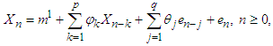
3.2. ARIMA Models
The basic processes of the Box–Jenkins ARIMA (p,d,q) model include the autoregressive process, the integrated process, and the moving average process. As part of the orientation of the research, fundamental definitions and notational conventions are specified, clarifying the mean and constant as well as the convention of the sign of moving average components. Our attention is then turned to the order of integration of the model, which is indicated by the I(d) distribution designation. If a series is I(0), then it is stationary and has an ARIMA(p,0,q) designation. If a series requires first differencing to render it stationary, then d=1 and it is distributed as I(1) and has an ARIMA(p,1,q) designation. Once the process has been transformed into stationarity, we can proceed with the analysis.In practice, to model possibly nonstationary time series data, we may apply the following steps:1. Look at the ACF to determine if the data are stationary.2. If not, process the data, probably by means of differencing.3. After differencing, fit an ARMA (p, q) model to the differenced data.Recall that in an ARIMA (p, d, q) model, the process {Yt} satisfies the equationTo see this, consider the following equation,Consider then an ARIMA (p, 1, q) process. With Wt=Yt−Yt−1, we have 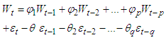 Or, in terms of the observed series,
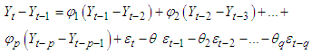
3.3. SARIMA
Suppose that {Yt} exhibits a seasonal trend, in the sense, To model this, consider where Such {Yt} is usually denoted by SARIMA (p, d, q) x (P,D,Q}S. Of course, we could expand the right-hand side of it and express {Yt} in terms of a higher-order ARMA model. But we prefer the SARIMA format, due to its natural interpretation. Structure for successive months in the same year and an ARMA structure for the same month in different years. Note accordingly, Yt also follows an ARMA model, with many of the intermediate AR and MA coefficients being restricted to zeros. Since there is a natural interpretation for a SARIMA model, we prefer a SARIMA parameterization over a long ARMA parameterization whenever a seasonal model is considered.This model is generally termed as the SARIMA (p, d, q) x (P,D,Q)S.For a seasonal time series of order s, [21] proposed that {Xt} be modeled by: A(L)Φ (Ls)∇dsXt = B(L) Θ(Ls)εtwhere the series must have been subjected to seasonal differencing D times and non-seasonal differencing d times, ∇s = 1 – Ls, being the seasonal differencing operator. Moreover Φ(L) and Θ(L) are the seasonal autoregressive and moving average operators respectively. These seasonal operators are polynomials in L. Suppose that Φ(L) = 1 + φ1L + φ2L2 + ... +φPLP and Θ(L) = 1 + θ1L + θ2L2 + ... + θQLQ, then the time series {Xt} is said to follow a multiplicative seasonal autoregressive integrated moving average model of orders p, d, q, P, D, Q and s, designated by (p, d, q)x(P, D, Q)s SARIMA model.Fit a subset SARIMA model. Find out if βs = 0. If so, the model is additive but if not, find out if the model is multiplicative. If not, the model is subset.
4. Results and Finding
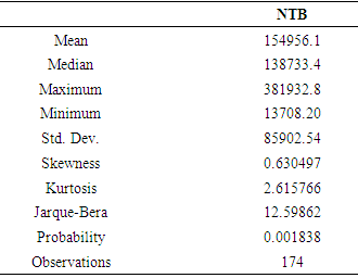
Tables and Figures of 91-day and 182 Treasury billTable 1. Descriptive Statistics of the Nigeria Treasury Bill data
 |
| |
|
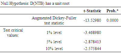
Table 2. Augmented Dickey-Fuller Test of stationarity (ADF) of the Nigeria Treasury Bill data
 |
| |
|
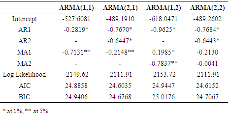
Table 3. Parameter Estimation of ARMA Models and Models selection
 |
| |
|
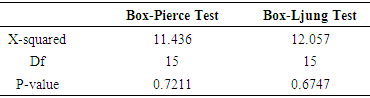
Table 4. Diagnostic tests for ARMA (2, 1) Model
 |
| |
|
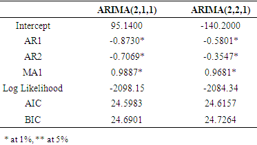
Table 5. Parameter Estimation of ARIMA Models and Models selection
 |
| |
|
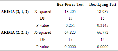
Table 6. Diagnostic tests for ARIMA Models
 |
| |
|
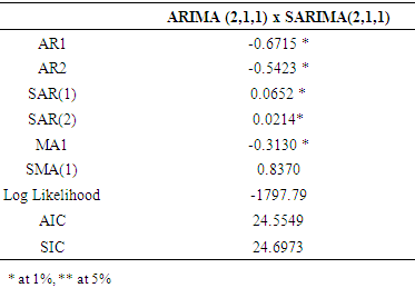
Table 7. Parameter Estimation of SARIMA Model
 |
| |
|
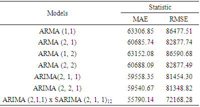
Table 8. Forecast Performance of estimated model of monthly Nigeria Treasury Bill
 |
| |
|
The stationarity of the Nigeria Treasury Bill data was investigated by observing the time plot of the series. The figure obtained as presented in graph 1 revealed that the series for Nigeria Treasury Bill data is not stationary but at first difference it is stationary as seen in graph 2. Using a statistic formula i.e. Augmented Dickey- Fuller Test. The statistic test shows that there is no unit root since it is less than critical values at 1% and 5% in Table 2. Table 3 shows the results of parameter estimation and model selection for the ARMA models, where results of the different estimation parameter of ARMA were estimated with most of the parameter significant at 1% and 5%. AIC was used to select the best model that will be used for ARIMA and SARIMA model because it is the combination of AR and MA model. From the AIC, ARMA (2, 1) was selected to be the best model since it has the smallest AIC. With this selection, our ARIMA model will be AR (2) and MA (1) while the integrated difference will be of one (1) and two (2). Using the best model in Table 3, the result of Table 4 shows the P-value for ARMA (2, 1) indicates there is no evidence that the residuals are dependent. This further confirms that the ARMA (2, 1) model is adequate. The Q-Q plot test was also adopted to test the residual whether is normally distributed, the plot test shows that the residual is normally distributed since the points in the plot lie close to the diagonal line, as shown in graph 3.We can now conclude that ARMA (2, 1) is a suitable model for this study of monthly Nigeria Treasury Bill. Table 5 shows the results of parameter estimation and model selection for the ARIMA models. The adequate model from the ARMA estimation was used to estimate the ARIMA model with integrated value of one (1) and two (2). Therefore, results obtained from the ARIMA model were significant at 1% and 5%, where the coefficient of AR is negative and MA is positive. AIC was used to select the best model, and from the AIC, ARIMA (2, 1, 1) was selected to be the best model since it has the smallest AIC than the ARIMA (2, 2, 1). However, this result will be used to compute the SARIMA model. The result on Table 5 shows the P-value for ARIMA (2, 1, 1) and ARIMA (2, 2, 1). The results of the p-values indicate that, there is no evidence that the residuals are dependent for ARIMA (2, 1, 1) while ARIMA (2, 2, 1) shows evidence of residual dependent. This confirms that the ARIMA (2, 1, 1) model is adequate. The Q-Q plot test was also adopted to test the residual whether it is normally distributed, the plot test shows that the residual is normally distributed since the points in the plot lie close to the diagonal line, as shows in graph 4 while ARIMA (2, 2, 1) model is not adequate with prove from the Q-Q plot test done.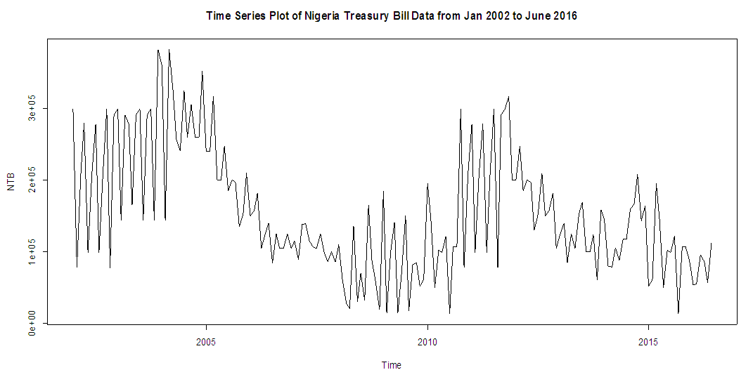 | Graph 1. Graph of monthly Nigeria Treasury Bill raw data |
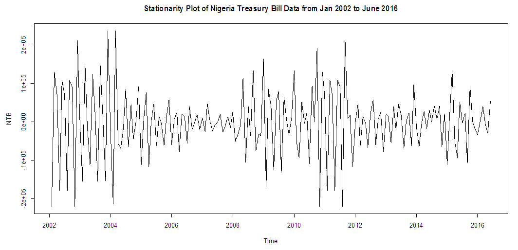 | Graph 2. Stationary plot of the series at first difference |
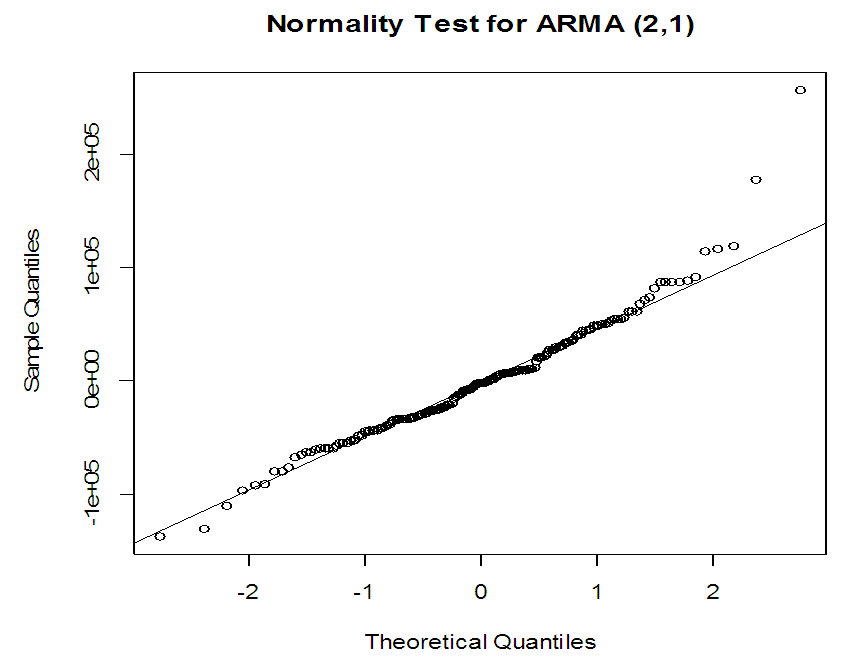 | Graph 3. Q-Q plot for ARMA (2, 1) model |
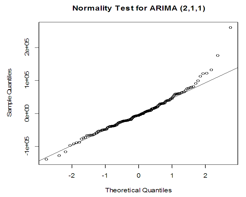 | Graph 4. Normality test for ARIMA (2,1,1) |
We can now conclude that ARIMA (2, 1, 1) is a suitable model of this study of monthly Nigeria Treasury Bill, the parameter estimation of SARIMA was computed as the results of the model selection and diagnostics test of the ARMA and ARIMA model where computed above. The results of parameter estimation for ARIMA (2, 1, 1) x SARIMA (2, 1, 1)12 models are significant at 1%. AIC was used to select the best model. From the AIC, ARMA (2, 1, 1) was selected to be the best model since it has the smallest AIC than the ARIMA (2, 2,1). The result on Table 7 shows the P-value for ARIMA (2, 1, 1) x SARIMA (2, 1, 1)12 of monthly data. The p-value indicates that there is no evidence that the residuals are dependent for ARIMA (2, 1, 1) x SARIMA (2, 1, 1). The Q-Q plot test was also adopted to test the residual whether is normally distributed, the plot test shows that the residual is normally distributed since the points in the plot lie close to the diagonal line. We can now conclude that ARIMA (2, 1, 1) x SARIMA (2, 1, 1)12, is a suitable model of this study of monthly Nigeria Treasury Bill.
5. Forecasting Evaluation of the Forecasting Models
Forecasting performance of these estimated forecasting models were investigated using our sample data and statistics like Mean Absolute Error and Root Mean Square Error. Model with the smallest Mean Square Error was considered to the most suitable for forecasting. Hence, from the results obtained in Table 8, it was observed that ARIMA (2, 1, 1,) x SARIMA (2, 1, 1)12 is the best forecasting model followed by ARIMA (2, 2, 1), ARIMA (2, 1, 1) models but ARIMA (2, 2, 1) is considered to be inadequate model from the diagnostic test. Therefore, the best forecasting models for monthly Nigeria Treasury Bill are ARIMA (2, 1, 1) x SARIMA (2, 1, 1)12 and ARIMA (2, 1, 1) models.
6. Conclusions
This study had come out with some findings in the comparing of forecasting models on monthly Nigeria Treasury Bill. From the results of the forecasting models, ARMA (2, 1), ARIMA (2, 1,1) and ARIMA (2, 1, 1) x SARIMA (2, 1, 1)12 are the adequate forecasting model in estimating Nigeria Treasury Bill. Furthermore, in terms of forecasting accuracy, the forecasting models were evaluated using the RSME and from the results, ARIMA (2, 1, 1) x SARIMA (2, 1, 1)12 is most suitable for forecasting. Moreover, using the forecasting models, it showed that for the next two years’ period, the Nigeria Treasury Bill will range below average of the normal issues from previous years, i.e. the predicted values for the rest of 2018 and 2019 are relatively close to the observed values. The post estimation evaluation carried out revealed various estimating models to be most suitable for monthly Nigeria Treasury Bill. The ARMA (2, 1), ARIMA (2, 1, 1) and ARIMA (2, 1, 1) x SARIMA (2, 1, 1,)12 was adequate in forecasting the monthly Nigeria treasury bill. But from the results of evaluation obtained, it was discovered that ARIMA (2, 1, 1) x SARIMA (2, 1, 1)12 is the best forecasting model for monthly Nigeria Treasury Bill Data. And It can also be concluded that Nigeria Treasury Bill Rates follow the additive SARIMA model. It means that a current value of the time series depends on the past value of a month ago and that of a year ago of shocks or its error terms. This model has been shown to be adequate and could be used for the forecasting of Nigeria Treasury bill rates. However, efforts should be made to explore the possibility of models that better account for the variability in the time series.
References
| [1] | Dieboida and Li. (2006): Comparative Analysis of Performance of Equities (stock) and Treasury bills in Ghana. Kwame Nkrumah University of Science and Technology. |
| [2] | Teye-Okutu, E.M.K. (2011). Modelling and Forecasting Ghana’s inflation rates using Sarima models. A Thesis submitted to the Department of Mathematics, Kwame Nkrumah University of Science and Technology in partial fulfillment of the requirements for the award of M.Sc. in Industrial Mathematics. |
| [3] | Granger and Pesaran, (2000) Forecasting of energy production and consumption in Asturias (northern Spain) Energy 24 pp. 183-198. |
| [4] | Abramson and Finizza, (1995). Forecasting the S&P 500 index volatility International Review of Economics and Finance 6(4) pp.391-404. |
| [5] | Britton et al. (1998) Forecasting tourist arrivals in Barbados Annals of Tourism Research 22(4) pp 804-818 Enders W Applied Econometric Time Series, John Wiley & Sons Inc. 1998 Cashcraft Asset Management Limited (2013). “Treasury Bills www.cashcraft.com/index.php?option=com_content&view=article&id=3448&Itemid=157. |
| [6] | Leitch and Tanner. (2009) Time series forecasts of international travel demand for Australia, Tourism Management 23(4) pp 389-396. |
| [7] | Garbade., (2008), Forecasting Exchange Rate: Theory and Practice, The Henley Centre for Forecasting, London. |
| [8] | Abdoulaye Camara, Wang Feixing and Liu Xiuqin (2016) “Energy Consumption Forecasting Using Seasonal ARIMA with Artificial Neural Networks Models” International Journal of Business and Management; 11(5), 231-243. |
| [9] | Susan W. Gikungu, Anthony G. Waititu and John M. Kihoro (2015) “Forecasting inflation Rate in Kenya using SARIMA model” American Journal of Theoretical and Applied Statistics. 4(1): 15-18. |
| [10] | Sun N, Li Y, Wu F, Zheng C, Hou K and Wang K (2015). Predictive analysis of outpatient visits to a grade 3, class a hospital using ARIMA model. In: proceeding of the 2014 international symposium on information technology (ISIT2014). Dalian: CRC press, 285. |
| [11] | Fannoh, R., Orwa G., and Mung’atu J. K. (2014), “Modeling the Inflation Rates in Liberia: SARIMA Approach”, International Journal of Science and Research, 3, 1360-1367. |
| [12] | Eni, D. and Adesola, A. W. (2013). “Sarima Modelling of Passenger Flow at Cross Line Limited, Nigeria”. Journal of Emerging Trends in Economics and Management Sciences, 4(4)427 – 432.1779-1801. |
| [13] | Osarunwense, O. (2013). Applicability of Box-Jenkins SARIMA model in rainfall Forecasting: A Case study of Port Harcourt South-South Nigeria. Canadian Journal on Computing in Mathematics, Natural sciences, Engineering and Medicine, 4(1), 1-4. |
| [14] | Kumar Manoj and Anand Madhu (2012) “An Application of Time Series Arima Forecasting Model For Predicting Sugarcane Production In India” Business and Economics 81-94. |
| [15] | Muhammed Jamil, Safoora Akbar, Abdul Majeed Akhtar, Zaheer-ul Hassan Mir, Abu Bakar Pesaran and Skoura, (2002). “The Determination of the Order of an Autoregression.” Journal of the Royal Statistical Society, Series B, 41, pp. 190-195. |
| [16] | Hamidreza M. and Leila S. (2012). Using SARFIMA model to study and predict the Iran’s oil supply. International Journal of Energy Economics and Policy. 2(1) 41-49. |
| [17] | Box, G. P. and Jenkins, G. M. (1976). Time Series Analysis, Forecasting and Control. Holden-Day. San Francisco. CA. |

 Abstract
 Reference
 Full-Text PDF
 Full-text HTML