-
Paper Information
- Paper Submission
-
Journal Information
- About This Journal
- Editorial Board
- Current Issue
- Archive
- Author Guidelines
- Contact Us
International Journal of Statistics and Applications
p-ISSN: 2168-5193 e-ISSN: 2168-5215
2019; 9(6): 171-179
doi:10.5923/j.statistics.20190906.01

An Evaluation of Frequentist and Bayesian Approach to Geo-spatial Analysis of HIV Viral Load Suppression Data
 Abstract
 Reference
 Full-Text PDF
 Full-text HTML
Collins Odhiambo, Mukami Joy Kareko
Strathmore Institute of Mathematical Sciences, Strathmore University, Physical Address: Ole Sangale Road, Madaraka, Nairobi, Kenya
Correspondence to: Collins Odhiambo, Strathmore Institute of Mathematical Sciences, Strathmore University, Physical Address: Ole Sangale Road, Madaraka, Nairobi, Kenya.
| Email: |  |
Copyright © 2019 The Author(s). Published by Scientific & Academic Publishing.
This work is licensed under the Creative Commons Attribution International License (CC BY).
http://creativecommons.org/licenses/by/4.0/

In Kenya, approximately 1.5 Million people are living with HIV and 28,000 deaths are recorded annually as a result of AIDS related illnesses. The country was considered a priority country by UNAIDS when it launched a 90-90-90 strategy in 2014. The strategy aimed to diagnose 90 per cent of all HIV-positive persons, provide antiretroviral therapy (ART) for 90 percent of those diagnosed, and achieve viral suppression for 90 per cent of those treated by 2020. This study is motivated by the need to assess the 3rd 90; viral suppression for 90 per cent of those ART treated and seeks to evaluate the two statistical paradigms (Frequentist and Bayesian) that have conventionally been used for geo-spatial trends analysis. The use of Frequentist approach or Bayesian approach has been used previously to assess the prevalence and incidence of diseases; this study however, seeks to compare the two approaches when analyzing spatial trends of HIV viral load suppression in Kenya. In revisiting the theoretical framework of the two approaches and application of real data from the Kenyan setting spanning from 2012 to 2017, results show the Bayesian approach as more robust and in depth and entailing more information when modeling spatial trends of viral load suppression. Further, first line ART regimen, HIV-TB co-infection and retention rates are significant predictors of viral load suppression.
Keywords: Viral load Suppression, HIV-TB co-infection, Bayesian approach, Frequentist approach
Cite this paper: Collins Odhiambo, Mukami Joy Kareko, An Evaluation of Frequentist and Bayesian Approach to Geo-spatial Analysis of HIV Viral Load Suppression Data, International Journal of Statistics and Applications, Vol. 9 No. 6, 2019, pp. 171-179. doi: 10.5923/j.statistics.20190906.01.
Article Outline
1. Introduction
- In 2014, United Nations Program on HIV/AIDS (UNAIDS) launched the 90-90-90 strategy whose aim was to achieve 90 per cent suppression among the HIV infected persons, to ensure that 90 per cent of the HIV infected people were under antiretroviral (ARV) treatment, and ensure that 90 per cent of all HIV infected persons were diagnosed and therefore aware of their status by 2020 [1]. It is estimated that about 1.5 million Kenyans were living with HIV in 2016 [2] whereas an estimated 71,034 new infections were recorded among adults (Age 15+), and 6,613 new infections recorded among children (Ages 0-14) in that same year [3]. This translates to a prevalence rate of about 7 per cent for women, who are most vulnerable to HIV infections and 4.7 per cent for men. The most affected county was Homa Bay; whose prevalence rate stood at 26 per cent. HIV contributes to 29 per cent of annual adult deaths, 20 per cent of maternal mortality and 15 per cent of deaths of children under the age of five years [1]. Treatment for HIV involves a combination of different ARV drugs, which prevent the virus from replicating by maintaining the immunity levels of the person while slowly reducing the replication of the virus in the body [4]. Administration of ARV drugs therefore reduces the viral load (VL) content per millimeter of blood suppressing the virus, subsequently slowing down progression of HIV to AIDS [5]. This can prevent transmission of the HIV virus to uninfected partners [6]. The HIV virus attacks the immune system cell in the body, known as CD4 helper lymphocyte cells, making the body unable to fight other infections [4]. Administration of ART will suppress the virus, reducing it to an almost undetectable level. This study seeks to evaluate the suppression rates among children and adults and also establish the percentages of this population which has the virus under control due to the administration of the ART. We specifically will focus on the trends in the suppression rates while trying to model the predictors of viral suppression. On the other hand, geo-spatial approaches have been used extensively in epidemiology for disease surveillance and intervention monitoring. Through mapping, governments have been able to identify disease spread and monitor the same, leading to proper control of epidemics such as trypanosomiasis in Africa [7,17,18]. However, Geographical Information Systems (GIS) have not been used extensively in the area of disease programming and disease monitoring indicators for HIV pandemic. Intrinsically, GIS has been employed largely to map diseases and show spread of outbreaks but not to show certain aspects of diseases such as retention, viral load monitoring and other, such, aspects useful in disease monitoring. This is the gap that this study is attempting to address. Further, no attempt has been made to compare Frequentist and Bayesian approaches on such disease monitoring indicators such as VL suppression. The aim is to model distributions and patterns of VL suppression using GIS and compare Frequentist and Bayesian Approaches. Specifically; we conduct location analysis by focusing on VL analysis and evaluate the patterns and HIV predictors with intention of analyzing health system complexities.
2. Material and Methods
2.1. Study Design
- The study population involved all HIV positive patients who were actively on ART from 2014 to 2017 as per NASCOP VL website (http://viralload.nascop.org/). Inclusion criteria included all facilities registered by the government of Kenya with MFL (Master Facility List) codes. Extracted data was assembled into a uniform excel format disaggregated by counties. The viral load data consisted of 3,123 sites that treated HIV adult and pediatric patients. The data collected also included other variables i.e. testing month, redrawn samples, 1st line patients, patients with HIV/TB co-infection and retention rate from January, 2014 to December, 2017 were extracted from the data warehouse. Areas of interest were; current suppression rates in different administrative counties in Kenya, current retention rates, correlation between retention and suppression rates, relationship between patients on first line treatment, HIV-TB co-infection rates and VL suppression rates and comparison of the current suppression rates as compared to the expected rates of suppression.
2.2. Study Area and Data Collection
- The study area covers all the 47 different counties in Kenya. Data was obtained from health centers at a county level which comprised of data including viral load tests, viral load results with > 1,000 mL/copies were collected retrospectively, by electronic abstraction from each site. Electronic data received was reviewed to ensure that each data element was correctly formatted and that all elements were captured. Data elements with incorrect formatting, unknown or incomplete information, or other inaccuracies were reviewed with the site and corrected. The data was combined across sites to achieve a uniformly constructed multi-site database. The study did not require any approval by the ethical review because we were using secondary data that is in the public domain.
2.3. Statistical Analysis
- Data was examined for viral load tested for patients on ART and virologic results were used to determine VL suppression. The primary area of interest was to analyze patterns of viral load suppression over the years. Given that the study sample was drawn from all facilities providing clinical care, individuals who were being initiated into the ART were likely to have the VL test together with those already on ART. Statistical analysis was performed using R Studio version 3.5.3.
2.4. Data Exploration and Visualization
- The dataset contained 10 variables namely; County, No. of facilities sending samples, rejected samples, redrawn tests, test, results with VL < 1000, Patients on 1st Line treatment, retention rates, patients with HIV-TB Co-infection and year in which these samples were obtained. An additional variable which was of interest was obtained by subtracting the results with VL < 1000 from the total tests obtained and then finding the percentage of the same so as to obtain the variable of individuals who were virally suppressed but as a percentage. This was done for each county and then done for each year from 2012 to 2017. Choropleth maps which show information by coloring each component area were used to provide an indication of the magnitude of the variable of interest which was then used as a means for visualizing this data over the same period of time.
2.5. Moran’s Index Statistic
- Moran’s I [8] was used to test the hypothesis that there was no spatial auto-correlation in the outcome variable and to measure the overall spatial auto-correlation. High Moran’s Index indicates that the data is highly correlated while the opposite is also true. The expected value of Moran’s I is −1/ (N − 1). Values of Moran’s I that exceed −1/ (N − 1) indicate positive spatial auto-correlation, in which the values are similar, whether high or low values are spatially clustered. Values of I below −1/ (N −1) indicate negative spatial autocorrelation, in which neighboring values are not similar [9].
2.6. Bayesian Approach
- Here we utilized the Conditional Autoregressive (CAR) Methods. CAR models propose conditionally autoregressive priors (CAR priors) in an empirical Bayes setting instead of the joint prior distribution. In addition, Breslow and Clayton [10] applied CAR priors as random effects distributions within likelihood approximations for Generalized Linear Mixed Models. CAR models have a specified conditional mean and variance;
 | (1) |
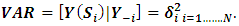 | (2) |
 denotes spatial dependence parameters. The primary purpose of CAR models is to provide a modeling mechanism to account for residual spatial correlation not explained by spatial patterns in covariate values. A number of different CAR prior models have been proposed in a disease mapping context and in the case disease monitoring indicators. We apply a combination of intrinsic model and a set of random variables as proposed by Besag et al [11]. The model is given by;
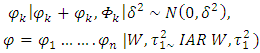 | (3) |
 ,
,  is not always possible. The MCMC convergence is also slow for this model. The CAR prior has the same conditional variance as the intrinsic model, while the conditional expectation is a weighted average of the mean of the random effects in neighboring areas and an overall mean µ.
2.7. Frequentist Approach
- In this approach, unlike the Bayesian approach, we made use of the data only and thereafter mapped it to find the results. In this approach, we analyzed the data and came up with an additional variable on ‘persons who are non-suppressed’ and later used the same to map the data and counties were used as the reference for the same. Chloropleth (maps that are shaded with different color intensities) were then used to show the same across all the counties in the country. After fitting the data, comparison of models enabled us choose the best model. In this study, we used the DIC and AIC to assess the fitness of a model, whereby the model with the least DIC was chosen as the best fit.
3. Results
3.1. HIV Viral Load Cases
- The 2012 to 2017 data on viral load suppression increased gradually over time from 116 centers to 2122 centers in 2017 submitting information on viral load. This also meant that the number of people being tested was increasing over time. Samples sent in, that were virally suppressed also increased significantly over time as shown below, as well as the number of tests that were taken over the years. The number of samples taken does not necessarily equal the number of people who visited the clinical facilities as one individual may have walked into the facility many times in that particular year or may have visited another clinic over the years.
|
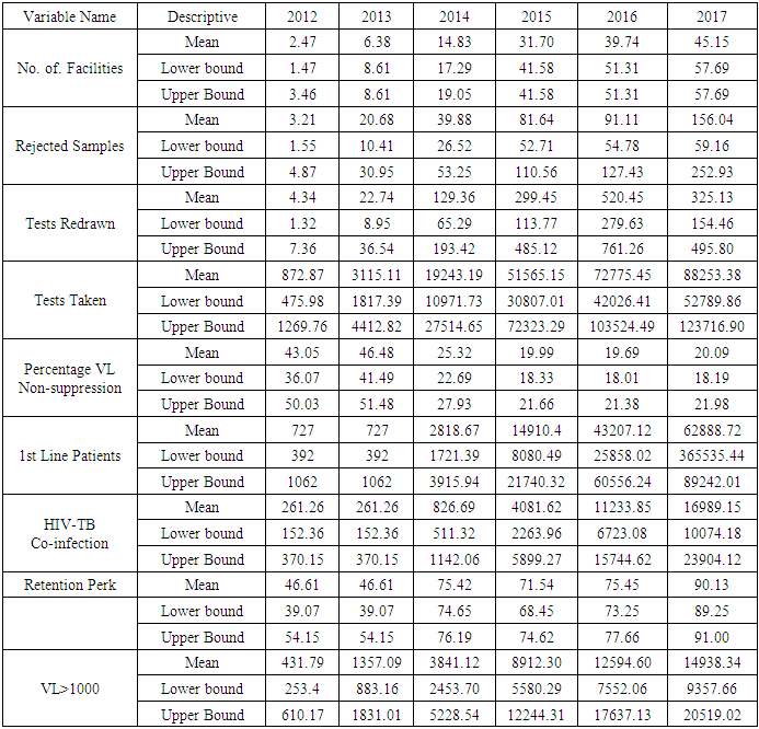
3.2. Results from Frequentist Approach
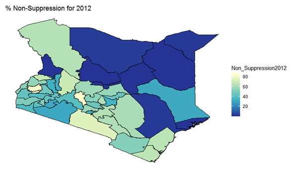
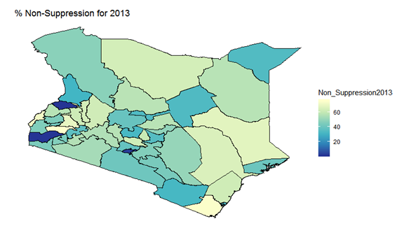
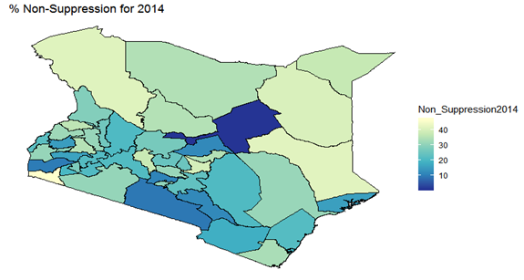
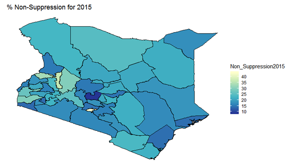
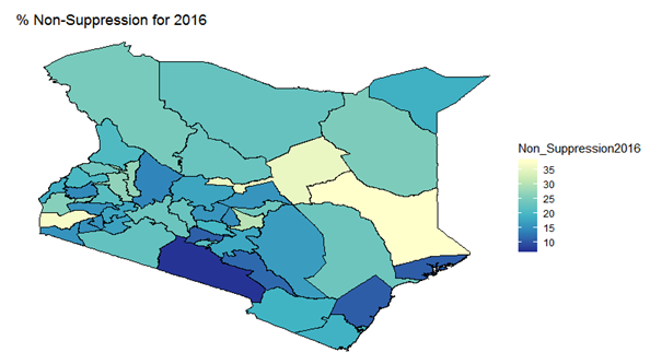
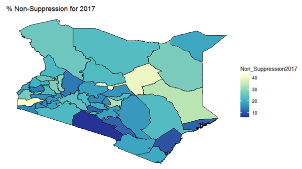
- By examining the data at county level, and plotting non-suppression rates, results show that in 2012, the counties that had the highest number of virally non-suppressed persons were, Nyandarua, Kakamega, Vihiga, Kajiado and Transzoia Counties. These counties also had the highest retention rates in that same year. However, in terms of HIV-TB co-infection, Nairobi, Kericho, Machakos, Kisumu and Homa Bay had highest numbers of infected individuals as well as the highest numbers of patients on 1st Line. Further, very few facilities were sending samples on VL across the country (only 116). This is partly because VL measurement had just been introduced as a HIV disease monitoring parameter. In that same year, counties such as Lamu, West Pokot, Mandera, Tana River and Isiolo did not have any facility that monitored VL and were therefore not recording VL suppressed samples. In 2013, there were some changes in counties which were least suppressed with Nyamira being at the top followed by Meru, Vihiga, Kakamega and Isiolo. Counties such as Kisumu and Busia had high rates of viral suppression. However, Mandera, Wajir and Samburu still had no entries on VL. Most patients on 1st Line were from Kiambu, Kisumu, Uasin Gishu, Busia and Nairobi. The same counties topped in the number of patients with HIV-TB co-infection. In terms of retention, counties such as West Pokot, Uasin Gishu, Mombasa, Tharaka Nithi and Kisii had the most numbers. There was also an increase in centers that measured the VL from 116 in 2012 to 300 in 2013. This was due to awareness created steadily over the period and an increase in donor funding in that same period from 18.85 per cent in 2012 to 19.6 per cent in 2013 [12,21,22]. In 2014, 626 centers sent samples on VL, while counties such as Turkana, Mandera, Tharaka Nithi, Wajir and Samburu were the least virally suppressed as compared to Kiambu, Vihiga, Busia, Migori and Kwale whose suppression rates were high. Centers sending the samples increased as well, owing to more awareness and availability of funds in these areas. Lamu, however, did not send any samples on VL that year as opposed to the previous year, 2013. This inconsistency was attributed to limited awareness on the importance of VL monitoring and poor infrastructure. In 2015, we observed that the centers sending the samples grew to 1490, as compared to centers in 2014. Counties such as Baringo, Wajir, Samburu, Turkana and April 26, 2019 8/16 Mandera were least suppressed. Population’s density in these counties is relatively low and may therefore not necessarily mean that these counties were doing poorly. However, counties such as Kiambu, Nairobi, Nyeri, Kirinyaga and Meru had high numbers of suppression rates, meaning that most samples sent had VL of less than 1000 copies/mL of blood. Further, Migori, Siaya, Homabay, Kisumu and Nairobi counties had the highest numbers of individuals with HIV-TB co-infections as well as patient’s on1st Line treatment. High retention rates were observed in Meru, Kirinyaga, Nyeri, Nairobi and Kiambu counties. We also observed that these counties were among the ones whose population was suppressed. In 2016, the facilities that were sending samples on VL rose 185 to 1868, as compared to 1426 in 2015. Retention rates in Nyandarua, Kiambu, Migori, Meru and Kirinyaga were highest. This meant that most of the patients in these counties continued in the treatment in that particular year. Population in Counties such as Turkana, Samburu, Mandera, Tana River, and Elgeyo Marakwet were most suppressed as opposed to people in Kirinyaga, Meru, Migori, Kiambu and Nyandarua counties. More so, Nairobi, Kisumu, Homa Bay, Siaya and Migori had the highest number of persons on 1st Line treatment as well as HIV-TB Co-infection. In 2017, the total number of facilities that sent the samples was 2122. This was approximately 13 per cent increase from 2016 and over 170 per cent from 2012. Nyeri, Kiambu, Kirinyaga, Muranga, Kisii had highest retention rates as compared to Elgeyo Marakwet, Mandera, Tana River, Samburu, Turkana which had least retention rates. Nairobi, Homa Bay, Kisumu Siaya and Migori had highest number of people with HIV-TB co-infection as well as patients on 1st Line treatment. In terms of suppression, Samburu, Turkana, Tana River, Mandera and Elgeyo Marakwet counties are least suppressed. High retention did not necessarily mean high suppression rates as will be clearer in the Bayesian Approach. Below maps show the regions that are least virally suppressed.
 | Figure 1. Map of non-suppression 2012 |
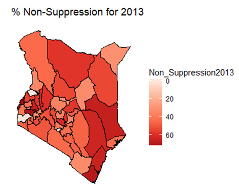 | Figure 2. Map of non-suppression 2013 |
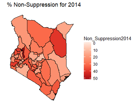 | Figure 3. Map of non-suppression 2014 |
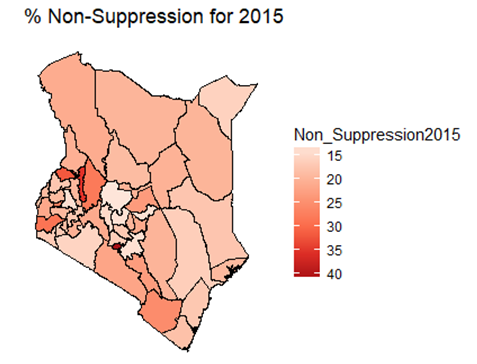 | Figure 4. Map of non-suppression 2015 |
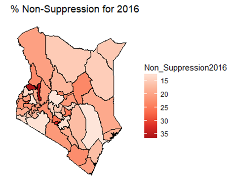 | Figure 5. Map of non-suppression 2016 |
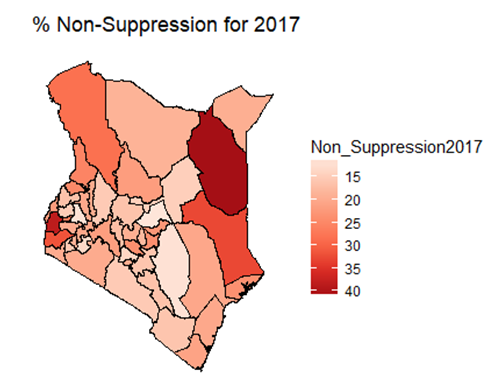 | Figure 6. Map of non-suppression 2017 |
3.3. Results from Bayesian Approach
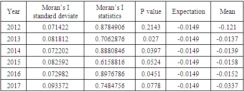
- Under the Bayesian paradigm, we employed spatio-temporal models in order to provide insight of counties high non-suppression. This provided a further analysis of predictors of non-suppression. Spatial auto-correlation was also measured to assess the extent of the existence of auto-correlation in the data using the global Moran’s I statistic. The table below shows that the data was spatially auto correlated owing to the small probability value (p-values) except in 2012, where the p-value was high. Existence of spatial autocorrelation meant that counties close to each other had almost similar outcomes as compared to those further from each other. Below is a summary of the findings;
|
 | Figure 7. Bayesian: non-suppression 2012 |
 | Figure 8. Bayesian: non-suppression 2013 |
 | Figure 9. Bayesian: non-suppression 2014 |
 | Figure 10. Bayesian: non-suppression 2015 |
 | Figure 11. Bayesian: non-suppression 2016 |
 | Figure 12. Bayesian: non-suppression 2017 |
4. Discussion
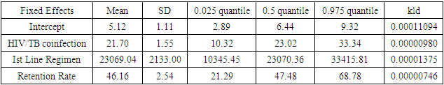
- In this study, we have assessed the spatial distribution of VL suppression in Kenya at different counties from 2012 to 2017. In addition, we have identified areas with high VL non-suppression using Bayesian smoothed maps, and Global Moran’s I statistics and the Frequentist approach. We also modeled the covariates that had an influence on VL non-suppression. For exploratory spatial data analysis, Bayesian smoothed maps of standardized non-VL suppression were generated. Standardized non-VL suppression was modeled to obtain accurate rates, and for comparison. This is because; areas with lower population might have indicated high suppression as compared to high population areas. This is one weakness of the Frequentist approach that Bayesian approach covered. This allowed visualization of spatial VL suppression patterns in 47 counties in Kenya. Results showed that Homabay, Isiolo and Garissa were least virally suppressed in 2017. In addition, most of the urban areas that recorded high viral suppression rates, such as Nairobi and Homabay are still highly non-suppressed for 2 consecutive years. Homabay’s high suppression rate is attributed to the fishing that goes on in the area. Mostly, residents in the area engage in sexual activities in exchange for fish, a popular delicacy in that area. Other factors may be due to movement of residents from Kenya to Uganda and Tanzania, which may be attribute to low retention and therefore adherence is poor. Wife inheritance, a popular practice in Homabay and which has been in place since independence could be one of the reasons for the low suppression rates despite the practice becoming unpopular. Usually, multiple sex partners can contribute to a new HIV strain that may require a different HIV regimen altogether. Isiolo and April 26, 2019 12/16 Garissa are popular counties of occupation for the Borana, Somali and Meru people. The high HIV non-suppression rate is attributed to low literacy levels, currently rated at 8 per cent by a Kenya National Adult Literacy Survey report. This report also indicated that Nairobi County had the highest literacy levels, leading to low and high awareness respectively. Global Moran’s I for spatial auto-correlation computed showed that counties closer to each other had similar relative VL non-suppression as compared to those further away. This relationship is significant in 2013 to 2017. We were also able to detect areas of decreasing or increasing trends of VL suppression in relationship to their neighbors. The Bayesian regression was also fitted to determine predictors of VL non-suppression. From the results, the 3 factors HIV/TB co-infection, 1st Line regimens and retention rates were significant. kld is interpreted as p-value. The model has nonrandom effects, no hyper parameters. The expected number of effective parameters was (stddev): 13.46(0.00), with number of equivalent replicates 113.30, deviance Information Criterion: 354.48, effective number of parameters: 4.973 and marginal likelihood:-336.0. See table below
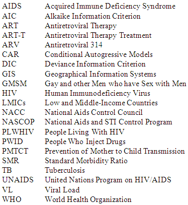
Abbreviation
References
| [1] | Luchuo Engelbart Bain, Clovis Nkoke, Jean Jacques N, BMJ Clobal Health, “Can the UNAIDS 90–90–90 target be achieved? A systematic analysis of national HIV treatment cascades”, March 7 2017, https://www.ncbi.nlm.nih.gov/pmc/articles/PMC5435269/. |
| [2] | Nall Rachel, September 2016 How HIV affects the body. Retrieved from Health line: www.healthline.com. |
| [3] | National Aids Control Council Kenya HIV County Profiles 2016. Nairobi; Kenya How HIV affects the body, September 2016. |
| [4] | UNAIDS 2017 Data Book. |
| [5] | Mata, N. L., and Mao, L. (2016). Estimating antiretroviral treatment coverage rates and viral suppression rates for homosexual men in Australia. Sex Health. |
| [6] | Cohen MS, C. Y Prevention of HIV-1 infection with early antiretroviral therapy. N Engl J Med, 365:493-505, 2011. |
| [7] | Catherine G Geanuracos, MSW, Shayna D. Cunningham, PHD and Jonathan M Ellen, MD Use of GIS for planning HIV Prevention Intervention for High Risk youths, November 2007. |
| [8] | Li, Hongfei; Calder, Catherine A.; Cressie, Noel (2007). Beyond Moran’s I: Testing for Spatial Dependence Based on the Spatial Autoregressive Model”. Geographical Analysis. 39 (4): 357–375. |
| [9] | WALLER, L. AND GOTWAY, C. Applied spatial statistics for public health data. Wiley- Interscience., 2004 32. Breslow, N.E. and Clayton, D.G. (1993) Approximate Inference In generalized Linear Mixed Models. Journal of the American Statistical Association, 88, 9-25. |
| [10] | Besag J, York J, Mollie A. Bayesian image restoration with two applications in spatial statistics. Ann Inst Stat Math 1991; 43: 1–59. |
| [11] | Leroux B, Lei X, Breslow N. Estimation of disease rates in small areas: a new mixed model for spatial dependence. In: Halloran M, Berry D, editors. Statistical models in epidemiology, the environment and clinical trials. New York: Springer-Verlag; 1999. p. 135–78. |
| [12] | UNAIDS and The Henry J. Kaiser Family Foundation (2017) Financing the Response to HIV in Low and Middle Income Countries: International Assistance from Donor Governments in 2016. |
| [13] | Michael J. Mugavero, Andrew O. Westfall, Anne Zinski, Jessica Davila, Mari-Lynn Drainoni, Lytt I. Gardner, Jeanne C. Keruly, Faye Malitz, Gary Marks, Lisa Metsch, Tracey E. Wilson, Thomas P. Giordano, Retention in Care (RIC) Study Group Measuring Retention in HIV Care: The Elusive Gold Standard, 2012 Dec 15; 61(5): 574–580. |
| [14] | Michael Carter TB doesn’t always increase HIV viral load, 06 January 2009, http://www.aidsmap.com/TB-doesnt-always-increase-HIV-viralload/page/1432925. |
| [15] | Jepchirchir Kiplagat,Ann Mwangi, Alfred Keter, Paula Braitstein Retention in care among older adults living with HIV in western Kenya: A retrospective observational cohort study. |
| [16] | C. W. (2016) Fact book, C. W. (2016). List of countries by HIV/AIDS adult prevalence rate. World Fact book 17. Kayvon Modjarrad, Sten H Vermund Effect of treating co-infections on HIV-1 viral load: a systematic review, Lancet Infect Dis. 2010 Jul; 10(7): 455–463. |
| [17] | Rashmi Kandwal Health GIS and HIV studies: Perspective and Retrospective, Journal of Biomedical Informatics, August 2009, pages 748-755. |
| [18] | Clarke KC, Mclafferty SL, Tempalski BJ On epidemiology and geographic information systems: a review and discussion of future directions, 1996 April 26, 2019 14/16. |
| [19] | Benjamin Young, September 10, 2014. The importance of retention in HIV care. |
| [20] | Gadner EM, McLees MP, Steiner JF, Del Rio C, Burman WJ. 2011 The Spectrum of engagement in HIV care and its relevance to test and treat strategies for prevention of HIV infection, 52:793-800. |
| [21] | Ministry of Health/National Aids Control Council, 2016 Kenya AIDS Response Progress Report Ministry of Health/National Aids Control Council, 2016. |
| [22] | US Department of Health and Human Services, March 2018, Viral Suppression among Youth and PWID is improving but results are still below the National Average: www.hiv.gov. |
| [23] | E Casetti, C.C. Fan The Spatial Spread of the AIDS epidemic in Ohio:empirical analysis using the expansion method, 1991, pg 1589-1608. |
| [24] | Boerma, R. S. Suboptimal viral suppression rates among HIV infected children in low and middle income countries; a meta-analysis. Clinical Infectious Diseases, 1645-1654 2016. |
| [25] | CDC. (2017, July 27) More People with HIV have the virus under control. Retrieved from Centers for Disease Control and Prevention: https://www.cdc.gov. |
| [26] | Ickovics J, M. C. Adherence to HAART among patients with HIV: breakthroughs and barriers. AIDS Care, 14:9-18, 2002. |
| [27] | UNAIDS. (2015). Biomedical Aids Research: Recent and Upcoming Advances: www.healthline.com. |
| [28] | UNAIDS 2017 Ending AIDS: Progress towards the 90-90-90 targets. April 26, 2019 15/16. |
| [29] | UNAIDS Factsheet-Latest statistics on the status of the AIDs epidemic, 2017. |
| [30] | UNAIDS The Global HIV/AIDS Epidemic. USA: UNAIDS, November 20, 2017. |