-
Paper Information
- Previous Paper
- Paper Submission
-
Journal Information
- About This Journal
- Editorial Board
- Current Issue
- Archive
- Author Guidelines
- Contact Us
International Journal of Statistics and Applications
p-ISSN: 2168-5193 e-ISSN: 2168-5215
2019; 9(5): 160-169
doi:10.5923/j.statistics.20190905.05

An Account of Principal Components Analysis and Some Cautions on Using the Correct Formulas and the Correct Procedures in SPSS
 Abstract
 Reference
 Full-Text PDF
 Full-text HTML
Dimitris Hatzinikolaou1, Katerina Katsarou2
1University of Ioannina, Department of Economics, Ioannina, Greece, and Hellenic Open University, 18 Aristotelous, Patras, Greece
2Technische Universität Berlin, Service-centric Networking, Telecom Innovation Laboratories, Berlin, Germany
Correspondence to: Dimitris Hatzinikolaou, University of Ioannina, Department of Economics, Ioannina, Greece, and Hellenic Open University, 18 Aristotelous, Patras, Greece.
| Email: |  |
Copyright © 2019 The Author(s). Published by Scientific & Academic Publishing.
This work is licensed under the Creative Commons Attribution International License (CC BY).
http://creativecommons.org/licenses/by/4.0/

The paper provides an account of the principal components regression (PCR) and uses some examples from the literature to illustrate the following: (1) the importance of PCR in the presence of multicollinearity; (2) some cautions on its correct implementation in SPSS, as some researchers use it improperly; (3) the use of the correct formulas, in accordance with the choice of scaling the variables; (4) the choice of principal components to be dropped; (5) the conditions for the PCR to outperform ordinary least squares, in the minimum mean-square-error sense; and (6) the robustness of the estimates to substantial changes in the sample.
Keywords: Multicollinearity, Principal Components, MSE, SPSS
Cite this paper: Dimitris Hatzinikolaou, Katerina Katsarou, An Account of Principal Components Analysis and Some Cautions on Using the Correct Formulas and the Correct Procedures in SPSS, International Journal of Statistics and Applications, Vol. 9 No. 5, 2019, pp. 160-169. doi: 10.5923/j.statistics.20190905.05.
Article Outline
1. Introduction
- A problem that is frequently encountered in applied regression analysis is multicollinearity, i.e., high correlation among the explanatory variables (regressors), which causes the estimates to be imprecise, thus leading to erroneous inferences and imprecise forecasts. As Jackson (2003, p. 276) notes, a “salvation in some thorny regression problem” of this type may be achieved by using principal components (PCs) analysis. Unfortunately, however, some researchers often fail to implement it properly, despite the strong warnings that exist in the literature; see, e.g., Jolliffe (1982) and Hadi and Ling (1998). For example, in a well cited paper, Liu, et al. (2003) drop the regressors that are not statistically significant at the 5-percent level before applying the principal components regression (PCR). This can lead to a wrong model, however, thus causing an omitted-variable bias, when in fact multicollinearity is to blame for the low values of the t-statistics, which, therefore, should not be taken to mean that the corresponding regressors are irrelevant (Chatterjee and Hadi, 2006, p. 299). Also, Liu, et al. (2003) erroneously interpret the “component matrix” (produced by the SPSS Factor Analysis procedure) as the matrix of eigenvectors, which can be obtained by writing a program, or by modifying the “component matrix” (see section 3). Apparently, as Sharma (1996, p. 58) notes, this confusion often arises in packages where principal component analysis is embedded in the factor analysis procedure. Finally, instead of using only a subset of the PCs in the model, Liu, et al. (2003) use all of them. Unless other errors are made, however, this procedure will return the original regression, thus nullifying the whole effort of implementing the PCR. Despite these errors, researchers still use Liu, et al. (2003) as a basic reference for the PCR, however; see, e.g., Ding, Ma, and Wang (2018) and Tran, et al. (2018).The present paper provides an account of the PCR (Section 2) and shows (in Section 3) step-by-step how to implement it correctly in SPSS by replicating an example from Chatterjee and Hadi (2006). We choose to replicate an example from a standard textbook, rather than providing our own, in order to convince the reader that the steps taken here are the correct ones. The example demonstrates the importance of the PCR, as it produces estimates that have the expected signs and are statistically significant at the 1-percent level, whereas the ordinary least squares (OLS) regression fails in that respect. This result becomes stronger when we update the sample substantially. In addition, in Sections 2 and 4, we use two other data sets, one from Chatterjee and Hadi (2006) and another from Myers (1990), to illustrate other important aspects of the PCR, namely, the use of the correct formulas, in accordance with the choice of scaling the variables; the choice of PCs to be dropped from the PCR; and the conditions for the PCR to outperform OLS in the sense of the minimum mean square error (MSE) criterion. Section 5 provides a summary.
2. An Account of the PCR and Some Measures of Multicollinearity
2.1. Estimation of the Coefficients of Interest via the PCR
- Consider the standard linear regression model with k regressors, X1, ..., Xk,
 | (1) |
 | (1a) |
 is the best linear unbiased estimator (BLUE). To implement the PCR, we first write (1) in terms of standardized variables,
  | (2) |
 is the n×1 vector of the standardized response variable, whose i-th element is defined as
  , where
  is the sample mean of y and
  is its standard deviation, so that
  has zero mean and unit standard deviation;
  is a n×k matrix (without a column of 1’s) whose ij-th element is defined as
  , where
  is the sample mean of Xj and sj is its sample standard deviation (sj > 0), j = 1, ..., k, i = 1, ..., n; θ is k×1; and
  is a n×1 error vector whose i-th (unobserved) value is
  , where
  is the sample mean of ε. We assume that Equation (2) is correctly specified; the X’s are stochastic, but strictly exogenous, implying that
  , i = 1, ..., n; and
 , where σ2 > 0 and In is the identity matrix of order n. Note that the literature on the PCR almost invariably assumes non-stochastic regressors, but here we adopt the assumption of stochastic regressors, because: (1) it is more realistic; (2) it renders the results more naturally interpretable, in that they are viewed as conditional on the observed values of the regressors; and (3) it has been adopted by famous modern econometrics textbooks, such as Hayashi (2000), Stock and Watson (2003), and Wooldridge (2006). Under these assumptions, the OLS estimator of θ, denoted as
  is BLUE. The vector θ is related to the slope vector βs as follows: θj = (sj/sy)βj, j = 1, ..., k, or
 | (3a) |
 | (3b) |
 | (4) |
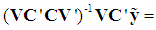
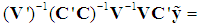
 can be written as
 | (5) |
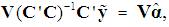
 is a k×1 vector of new coefficients, defined as
  , hence
  Thus, the OLS estimators of
  and
and  are related as follows:
 | (6) |
 = CV', and note that
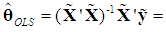
 since it is obvious from (5) that, when all the (k) PCs are retained, the OLS estimator of
  is
is  which, under the classical assumptions, is BLUE. Pre-multiplying (6) by V' and using V' = V-1 yields
  | (7) |
 and
and  that would be obtained by applying OLS to Equations (1)-(2), so it is of no practical interest, as the idea of the PCR is to escape from these imprecise estimators in the presence of multicollinearity. In practice, we always want to drop d PCs whose variances are close to zero or have no predictive power for
  in (5), and hence also drop the corresponding d columns of V and the corresponding d elements of
  . Let
. Let  and
and  denote the resulting PCR estimators of θ and β, which are biased (Myers, 1990, p. 415). Thus, instead of (6), we want to have a relation between
  and the k – d retained elements of
  , collected in the (k-d)×1 sub-vector
  . Let
. Let  denote the d×1 sub-vector of the d dropped elements of
  , and partition V as
  where Vk-d is the k×(k-d) sub-matrix of the k-d retained eigenvectors, and Vd is the k×d sub-matrix of the d dropped eigenvectors. Thus, (6) is replaced by
 | (8) |
 , and hence, using Equation (3b),
  ; see Chatterjee and Hadi (2006, p. 264, Table 10.3, and p. 231, Table 9.7) and Rawlings (1988, p. 360). Finally, since
 is the covariance matrix of the k PCs, where λ1, ..., λk are the eigenvalues of the correlation matrix of the regressors,
  (Hadley, 1961, p. 248), it is useful to partition Λ as follows:
 | (9) |
 are diagonal matrices of order k-d and d, respectively, whose elements in the main diagonal are the eigenvalues associated with the retained and the dropped PCs, respectively; the upper-right zero sub-matrix is (k-d)×d, and the lower-left one is d×(k-d). Note that, since
  is positive definite, it follows that λ1 > 0, ..., λk > 0 (Goldberger, 1964, p. 34), so
  is also positive definite, and so are
  Applying the result of inverting a partitioned nonsingular matrix to (9) (Hadley, 1961, pp. 107-109), we can now write the OLS estimator of
  as follows:
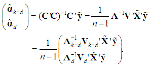 | (10) |
2.2. Variance of  and
and  , t-ratios, Bias, and Mean Square Error
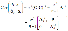
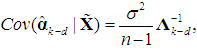
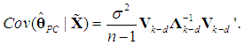
- Consider the variance-covariance matrix of
 obtained from (8),
 | (11) |
 | (12) |
 | (13a) |
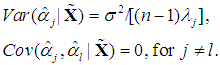 | (13b) |
 | (14a) |
 | (14b) |
 (and hence of
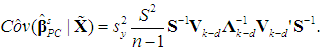
  ) may be inflated. Note that, since we use Chatterjee and Hadi’s (2006, p. 240) second type of scaling the variables in (2), which are standardized with zero mean and unit standard deviation (not unit length); and since the λ’s are the eigenvalues of the correlation matrix
 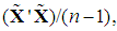 the division by n – 1 in (14b) is correct; see McCallum (1970), Cheng and Iglarsh (1976), and Gunst and Mason (1980, pp. 114-115). We stress this point, as the various types of scaling used in the literature seem to be a source of error. For example, in Chatterjee and Hadi’s (2006, pp. 249-251) application of the PCR to the advertising data, where the variables and the λ’s are defined as above, the authors fail to divide their Equations (9.34) and (9.35) by n – 1. Their calculation of the standard error of
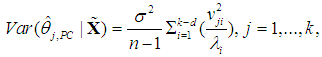
  is correct, however, as it is based on their Equation (9.33), which is correct.1Now, using (3a), we can write
 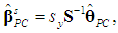 hence
hence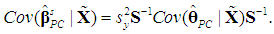 | (15a) |
 | (15b) |
 | (15c) |
 is the same as that of
  , j = 1, ..., k, since
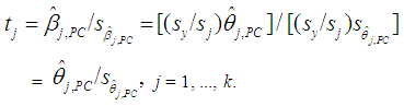 | (16) |
 (and hence
  ) is biased. To calculate its bias, we follow Myers (1990, p. 415) and begin by using (7), to obtain
  | (17a) |
 | (17b) |
 so
so  | (18) |
 is unbiased. Now, since VV' = I, we have that
  hence
hence  so (18) becomes
  =
= From (17b) we have
  Substituting in the previous equation yields
 so
so  | (19) |
 and
and  , we must determine whether the k×k matrix
  is positive semi-definite, in which case
  will be preferable. Since
  is unbiased, we have
  But, using (12), we obtain from (6) the following expression:
 Thus, we have
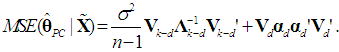
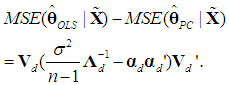
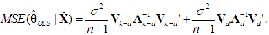 | (20a) |
 which is positive semi-definite, since Λd is positive definite and the k×d matrix Vd has rank d < k (Rencher and Schaalje, 2008, p. 26, Corollary 2). Thus, the variance of
  will never be greater than that of
  , so the burden of the choice between the two estimators falls on the size of the
 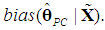 If the cost (bias) of falsely omitting a PC (underfitting) outweighs the gain (lower variance), the PCR will fail to be a minimum MSE estimator. By definition (see Goldberger, 1964, p. 129), we have
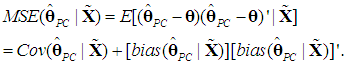 | (20b) |
 | (20c) |
 | (21) |
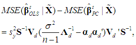 | (22) |
 and S is defined in (3a). The k×k symmetric matrix in (21) will be positive semi-definite if and only if all its eigenvalues are nonnegative (Goldberger, 1964, p. 37). Note that if the matrix in (21) is positive semi-definite, then so is that in (22), since the latter comes from the former by multiplying it by the positive scalar sy2 and by pre- and post-multiplying it by the positive definite matrix S-1 (see Hadley, 1961, p. 255). In fact, (21) and (22) will be positive semi-definite if
 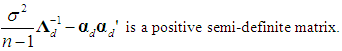 | (23) |
 | (24) |
 is a scalar, so it can be factored out in (21), and the kk matrix that emerges, VdVd', is positive semi-definite [Goldberger, 1964, p. 37, Property (7.15) with P = Vd']. Note also that versions of (23) already exist in the literature (see, e.g., McCallum, 1970, Farebrother, 1972, and Özkale, 2009). In particular, McCallum’s (1970, p. 112) condition (12) can be shown to be a special case of (23) for k = 2 and considering the MSE of only one coefficient. Consider the factors that enter (23) and favor the PCR over the OLS estimator. First, the larger the error variance (σ2) is, the more crucial it becomes to reduce the coefficient variances via the PCR. Second, for the same reason, the smaller the size of the sample (n), the higher the level of uncertainty, and hence the larger the need for precision of the coefficient estimates gained by applying the PCR. Third, the smaller the eigenvalues associated with the dropped PCs are, the more severe the multicollinearity problem is, hence the more meaningful the application of the PCR becomes. Fourth, the smaller the (absolute) values of the coefficients of the dropped PCs (
 ) are, the weaker the effects of these PCs on the dependent variable, and hence the more justifiable their removal from the PCR becomes. Note that a difficulty with condition (23) is that it involves unknown parameters. A way out is to use their unbiased estimators (see McCallum, 1970, p. 112, Farebrother, 1972, p. 335, and Özkale, 2009, p. 546). Since σ2 is inherited from Equation (2) or (5), its estimate (s2), as well as the estimate of
  , should be obtained from the regression equation (5) that retains all the PCs. In sum, we have the followingProposition 1:
  outperforms
  , in the minimum MSE sense, if and only if the eigenvalues of the symmetric d×d matrix
  are all nonnegative. Necessary (but not sufficient) conditions are
  j = 1, ..., d, where s2 and
  (an element of
  ) are obtained from regression (5) that retains all the PCs. As a test of dropping the “optimal” number of PCs, one can start from the PC with the smallest eigenvalue or from the most insignificant one in (5), and keep dropping PCs until the condition is violated. For d = 1, the condition is also sufficient.
2.3. Some Measures of Multicollinearity
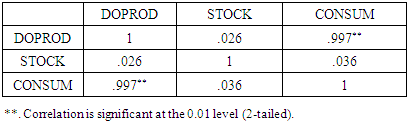
- The simplest measures of multicollinearity that one could think of are the absolute values of Pearson’s pairwise correlation coefficients (rij) among the regressors. If k = 2, this criterion is reliable, in that a “low” value of r12 means absence of multicollinearity and a “high” value of r12 means that multicolinearity is present. If k > 2, however, this criterion is not reliable, in that, although “high” values of rij (at least one of them) still imply that multicolinearity is present, nevertheless “low” values of rij do not necessarily imply absence of multicollinearity (Chatterjee and Hadi, 2006, pp. 233-237). Kmenta (1971, pp. 382-384) presents an example with k = 3, where there exists an exact linear relationship among the three regressors, i.e., there is perfect multicollinearity, and yet none of the three rijs exceeds 0.5 in absolute value.According to another simple criterion, multicollinearity is considered harmful if, at a level of significance, say, 5-percent, the standard F statistic (for the hypothesis that the joint effect of all the regressors is zero) is significant, but all the t-statistics for the individual slope coefficients are insignificant. As Kmenta (1971, p. 390) points out, however, this criterion is too strong, since it considers multicollinearity harmful only when all the t-statistics for the slopes are insignificant, which makes it difficult to disentangle the individual effects of the regressors on the dependent variable.Chatterjee and Hadi (2006, p. 233) suggest that researchers should pay attention to the following indications of multicollinearity: (i) large changes in the estimated coefficients if a regressor is added or dropped, or if a data point is altered or dropped; (ii) insignificant t-statistics for regressors that are important, according to the pertinent theory; and (iii) the signs of some of the estimated slope coefficients do not conform to those expected (based on theoretical grounds). A well-known statistic that measures multicollinearity is the variance inflation factor (VIF), defined as VIFj = 1/Tolerancej, where Tolerancej = 1 – Rj2 and Rj2 = the coefficient of determination in the (auxiliary) regression of Xj on the other regressors. Clearly, if the Xs are orthogonal among themselves, then Rj2= 0 and VIFj = Tolerancej = 1, j = 1, ..., k. According to Chatterjee and Hadi (2006, p. 238), “a VIF in excess of 10 is an indication that multicollinearity may be causing problems in estimation.” Another indication of the presence of multicollinearity is that some eigenvalues are close to zero. Thus, as another measure of multicollinearity, some authors suggest the condition index (κ), defined as
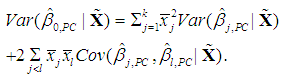
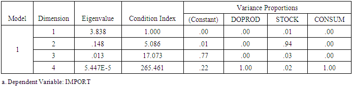
 where λ1 and λp are, respectively, the largest and the smallest eigenvalue of the matrix X'X. By definition, κ > 1. A large value of κ is evidence of strong multicollinearity, suggesting that the inversion of X'X will be sensitive to small changes in X. As an empirical rule, multicollinearity is considered to be harmful when κ > 15 (Chatterjee and Hadi, 2006, pp. 244-245).The diagnostics of multicollinearity are often complemented by the “variance proportions” in assessing the effect of each linear dependency among the regressors on the coefficient variances. In the OLS regression Equation (1), if any of the eigenvalues of X'X is close to zero (indicating a serious linear dependency), the variance of any or all of the coefficients in
  may be inflated. The variance proportion pji is the proportion of the variance of the coefficient
  attributed to the linear dependency characterized by the eigenvalue λj (see Myers, 1990, pp. 371-379).
3. Step-by-Step PCR in SPSS by Replicating and Updating an Example
- Chatterjee and Hadi (2006, ch. 9) illustrate the PCR by estimating a linear imports function using French annual aggregate data, 1949-1959 (n = 11), on Imports (IMPORT, y), Gross Domestic Product (DOPROD, X1), increase in Inventories (STOCK, X2), and Consumption (CONSUM, X3), all measured in billions of French francs at 1959 prices. Some useful descriptive statistics are
 =21.891,
  =194.591,
  = 3.3,
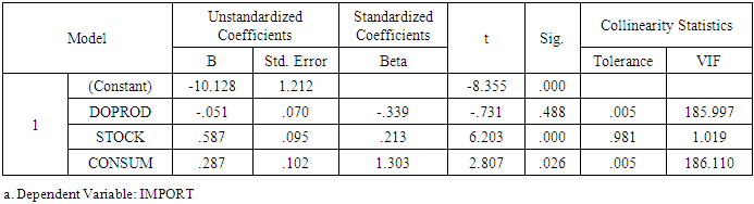
  = 139.736, sy = 4.5437, s1 = 30, s2 = 1.6492, and s3 = 20.6344.Note that in this example there are economic as well as econometric reasons to believe that the classical assumptions fail. For example, from the point of view of correct specification, instead of including STOCK and CONSUM as regressors, we would include the real exchange rate; and from the point of view of time-series econometrics, we would consider the problems of nonstationarity, endogeneity of the regressors, and serial correlation. We refrain from these issues here, however, and focus on the correct application of the PCR.In step 1, we apply OLS to Equation (1) and use the above criteria to decide whether multicollinearity is harmful. After entering the data in SPSS and selecting Analyze > Regression > Linear > Statistics > Collinearity Diagnosticswe get R2 = 0.992 (coefficient of determination) and Tables 1-2. The second and the fourth column of Table 1 report the elements of
  and
and  . Note that the coefficient
  = -0.051 has the wrong sign and is insignificant at all conventional levels (p-value = 0.488). Economic theory suggests that domestic income exerts a positive influence on imports, so we blame multicollinearity for these unexpected results, and keep DOPROD for the PCR.
|
|
 and
and  , namely, p31 = 0.9984 and p33 = 0.9989 (see Table 2, where both of these values are rounded to 1). That is to say, 99.84% of
  and 99.89% of
  can be attributed to the above linear dependency.
|
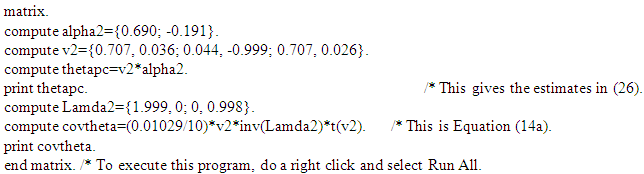
 by selecting File > New > Syntaxand by writing the following program in the command syntax window that appears:
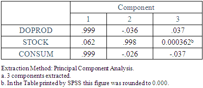
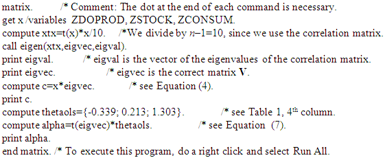 Although this program produces the correct matrix V directly, we will also construct it manually, in order to see the error made by Liu, et al. (2003). First, select Analyze > Dimension Reduction > Factor > (insert into the dialog box the variables) DOPROD, STOCK, CONSUM > Extraction > Fixed Number of Factors > Factors to Extract > (enter into the dialog box) 3 (the number of the original regressors) > Continue > OK. Tables 4-5 report the results. The 3×3 “component matrix” (Table 5) differs from that in Chatterjee and Hadi (2006, p. 243) and does not satisfy the property V'V = I, so it is not the correct matrix of eigenvectors, as Liu, et al. (2003) erroneously assume. Its elements need to be “normalized,” i.e., its columns must be divided by the square root of the corresponding eigenvalue, given by the second column of Table 4. That is, the first column of this matrix must be divided by
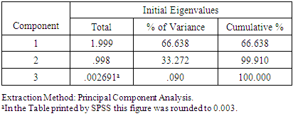
  the second by
  and the third by
  We thus obtain the correct matrix of eigenvectors:
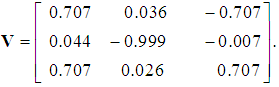 | (25) |
|
|
 and hence that of
  ; see Equations (14b), (15a)-(15c). If C3 is included in the regression equation (5), along with C1 and C2 (and no intercept), its coefficient is
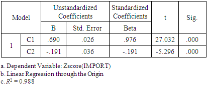
  = 1.16, which is insignificant at the 5-percent level (p-value = 0.095), whereas the other estimates are the same as those of Table 6. Thus, we estimate (5), using only C1 and C2 as regressors (and no intercept), implying that the third column of V in (25) is dropped.4 Table 6 reports the results.Equation (5) does not suffer from multicollinearity, since the PCs are orthogonal. The estimates
  and
and  (Table 6) have no natural interpretation, however, since the PCs are linear combinations of the original variables, so they are used only as an intermediate step to estimate the βs.
|
 and
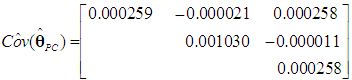
and  and their standard errors (s.e.). Using (8), where Vk-d is 3×2, and the above estimates of α1 and α2, we get
 | (26) |
 | (27) |
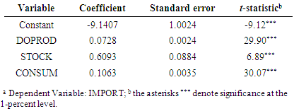
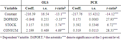
 Next, using (3b), we calculate the values of the
  These estimates are reported in Table 7 (the PCR) and are the same as those obtained by Chatterjee and Hadi (2006, p. 263).5 Table 7 also reports the estimated s.e.s of the
  and their t-ratios. The s.e.s are obtained from the matrix
  which is calculated in accordance with (15a)-(15c) and (27) and is reported below in (28) (the covariances between
  and the slope coefficients are not reported, as they are almost never useful):
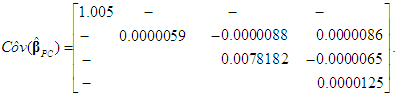 | (28) |
 = 1.16 is relatively large.
|
 and
and  are p31 ≈ p33 ≈ 0.9994. Thus, following exactly the same steps as before, we obtain and report the OLS and the PCR estimates side by side in Table 8.
|
 = -3.543, so 0.038767/(580.000873) – 3.5432 = -11.78 < 0. The failure of the minimum MSE criterion to support a theoretically and empirically sound result suggests that other criteria for comparing the PCR with the OLS estimator should also be used. This is beyond the purpose of this paper, however; see, e.g., Wu (2017).
4. Another Example, Where More than One PCs are Dropped
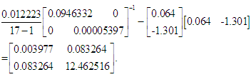
- To illustrate how Proposition 1 is implemented when more than one PCs (not necessarily consecutive) are to be dropped from the regression equation (5), we employ the “Hospital manpower data” given in Myer’s (1990, pp. 132-133) Table 3.8, where n = 17 and k = 5. In this example, too, multicollinearity is strong, as the bivariate correlation coefficients are high and highly statistically significant, e.g., r13 = 0.9999, r14 ≈ r34 ≈ 0.94, r12 ≈ r23 ≈ r24 ≈ 0.91, whose p-values for two-tailed tests are all 0.000; VIF1 = 9598 and VIF3 = 8933; the condition index is κ = 427; the last three eigenvalues of the X'X matrix are 0.0447, 0.0082, and 0.00002848; and the two highest variance proportions are p51 ≈ p53 ≈ 0.999. In this example, we have s2 = 0.012223; the last three eigenvalues of the correlation matrix are λ3 = 0.0946332, λ4 = 0.040712, and λ5 = 0.00005397; and the PCs C3 and C5 are statistically insignificant in (5), since the p-values of their estimated coefficients,
 = 0.064 and
  = -1.301, are 0.493 and 0.735 (whereas the p-values of the coefficients of C1, C2, and C4 are 0.000000, 0.000976, and 0.001859). Thus, if we drop C5 only, Proposition 1 gives
  | (29) |
 | (30) |
 outperforms
  in the minimum MSE sense.
5. Summary
- In this paper, we revisit the PCR and show step-by-step how to implement it properly in SPSS by replicating an example of Chatterjee and Hadi (2006), in which the regressors are highly collinear. The PCR proves to be important, as it produces estimates that have the expected signs and are statistically significant at the 1-percent level, whereas the OLS fails in that respect. This result becomes stronger when we update the sample substantially. Our main motivation has been the fact that some researchers still fail to implement this useful estimation method properly, despite the strong warnings that already exist in the literature. As an example of such a failure, we have briefly commented on the paper by Liu, et al. (2003). In addition, we use two more data sets from the literature to illustrate other important aspects of the PCR, namely, the use of the correct formulas, in accordance with the choice of scaling the variables, the choice of PCs to drop, and the conditions for the PCR to outperform OLS in the sense of the minimum MSE criterion.
Notes
- 1. The data for this example are given in Table 9.9 of Chatterjee and Hadi (2006, p. 236), where n = 22. Using the exact figures, and not the three-digit approximations used by the authors, we confirmed that the eigenvalues of the correlation matrix are indeed those given on p. 251, and that if their Equations (9.34) and (9.35) are used, then the standard error of
 is incorrectly calculated as 1.947. On the other hand, their Equation (9.33) and our Equation (14b) both give the correct estimate of this standard error, which is 0.425
  Note that Chatterjee and Hadi’s estimate of this standard error is given on p. 253 and is slightly different, 0.438, because of rounding errors.2. The proof of Equation (22) is given in an appendix that is available from the first author upon request.3. For an excellent theoretical discussion of the collinearity indices reported in Tables 2 and 3, including their marginal values, see Myers (1990, pp. 123-133, 369-371) and Rawlings (1988, pp. 273-281).4. The regressor sets {C1, C3}, {C2, C3}, {C2}, {C3} (and no intercept) all produce insignificant coefficients.5. Chatterjee and Hadi (2006, p. 263) report a slightly different estimate of the intercept, namely -9.106, apparently because of rounding errors.