Eleazar C. Nwogu1, Iheanyi S. Iwueze1, Kelechukwu C. N. Dozie2, Hope I. Mbachu2
1Department of Statistics Federal University of Technology, Owerri, Imo State, Nigeria
2Department of Statistics Imo State University, Owerri, Nigeria
Correspondence to: Kelechukwu C. N. Dozie, Department of Statistics Imo State University, Owerri, Nigeria.
| Email: |  |
Copyright © 2019 The Author(s). Published by Scientific & Academic Publishing.
This work is licensed under the Creative Commons Attribution International License (CC BY).
http://creativecommons.org/licenses/by/4.0/

Abstract
This study discusses the condition(s) under which the mixed model best describes the pattern in an observed time series data, while comparing it with those of the additive and multiplicative models. Existing studies have focused on how to choose between additive and multiplicative models, with little or no emphasis on the mixed model. The ultimate objective of this study is therefore, to propose a statistical test for choosing between mixed and multiplicative models when the trending curve is linear. in descriptive time series analysis. The method adopted in this study is the Buys-Ballot procedure developed for choice of model by [1]. Results show that the column/seasonal variance of the Buys-Ballot table is, for the mixed model, a constant multiple of the square of seasonal effect and for the multiplicative model, a quadratic (in j) function of the square of the seasonal effects. Therefore, test for the choice between mixed and multiplicative models has been proposed based on the column/seasonal variances of the Buys-Ballot table. have been used to illustrate the applicability of the proposed test, Using empirical examples, the proposed test statistic identified the mixed model correctly in 98 out of the 100 simulations.
Keywords:
Choice of Model, Time Series Decomposition, Mixed Model, Multiplicative Model, Buys-Ballot Table
Cite this paper: Eleazar C. Nwogu, Iheanyi S. Iwueze, Kelechukwu C. N. Dozie, Hope I. Mbachu, Choice between Mixed and Multiplicative Models in Time Series Decomposition, International Journal of Statistics and Applications, Vol. 9 No. 5, 2019, pp. 153-159. doi: 10.5923/j.statistics.20190905.04.
1. Introduction
One of the greatest challenges identified in the use of descriptive method of time series analysis is choice of appropriate model for decomposition of any study data. That is, when to use any of the three models for analysis is uncertain. And it is clear that; use of wrong model will certainly lead to erroneous estimates of the components.The three models most commonly used for time series decomposition are theAdditive Model: | (1) |
Multiplicative Model: | (2) |
and Mixed Model | (3) |
where for time t,  , is the observed time series,
  is the trend,
  is the seasonal effect,
  is the cyclical and
  is the irregular component [2,3].For short period time series data the cyclical component is superimposed into the trend and the observed time series
  can be decomposed into the trend-cycle component
  , seasonal component
  and the irregular/residual component
  , [3]. Therefore, the decomposition models areAdditive Model:
  | (4) |
Multiplicative Model:  | (5) |
and Mixed Model  | (6) |
It is always assumed that the seasonal effect, when it exists, has period s, that is, it repeats after s time periods. | (7) |
For Equation (4), it is convenient to make the further assumption that the sum of the seasonal components over a complete period is zero, ie, | (8) |
Similarly, for Equations (5) and (6), the convenient variant assumption is that the sum of the seasonal components over a complete period is s. | (9) |
It is also assumed that the irregular component  is the Gaussian
  white noise for Equations (4) and (6), while for Equation (5),
  is the Gaussian
  white noise and that
  On the most appropriate condition to use any of the three models, many scholars have proposed different approaches. [3] proposed the use of the run sequence plot (time plot) to choose between additive and multiplicative models. However, he did not provide any statistical test to justify the use. [4] proposed the use of the coefficients of variation of seasonal differences (CV (d)) and seasonal quotients (CV(c)) for choice of model. According to [4], the appropriate model is Additive if
  and Multiplicative if
  . However, neither the theoretical basis nor the statistical test was provided for the decision rule to justify the use. According to [5], the differences between the multiplicative and the additive models are (i) in the additive model, the seasonal variation is independent of the absolute level of the time series and its amplitude is relatively close while in the multiplicative model, the amplitude of the seasonal factor varies with the level of the time series; (ii) in an additive model, the seasonal effect is the same (roughly constant) in the same period over different years. Sometimes the seasonal effect is a proportion of the underlying trend value. In such cases it is appropriate to use a multiplicative model. No statistical test was provided for the choice. [6] proposed the use of the relationship between the seasonal means
  and the seasonal standard deviations
 , when data is arranged in a Buys-Ballot table, to choose the appropriate model for decomposition. According to [6], the appropriate model is additive when the seasonal standard deviations show no appreciable increase or decrease relative to any increase or decrease in the seasonal means. On the other hand, the appropriate model is multiplicative when the seasonal standard deviations show appreciable increase/decrease relative to any increase /decrease in the seasonal means. Here again, no statistical test was provided for the choice. From the foregoing, it is clear that there is no accurate statistical test for choice of model in the literature and the emphasis has been on choice between additive and multiplicative models. In the framework for choice of model and detection of seasonal effect in time series, [1] showed that when the trend-cycle component is linear, the column variances of the Buys-Ballot table are constant for the additive model, but contain the seasonal component for the multiplicative model. Thus, choice between additive and multiplicative models reduces to test for constant variance to identify the additive model. Therefore, they suggested that any of the tests for constant variance can be used to identify a series that admits the additive model. This is an improvement over what is in existence. However, this approach can only identify the additive model (when the column variance is constant), but does not tell the analyst the alternative model when the variance is not constant. The implication of this is that when the test for constant variance says the appropriate model for a study series is not the additive model; an analyst still faces the challenge of distinguishing between mixed model and the multiplicative model. Furthermore, in deriving, the row, column and overall averages and variances, [1] ignored the error term. Since the row, columns and overall averages and variances of the Buys-Ballot table are the bases for the proposal by [1] for choice between additive and multiplicative models; can they also be used to distinguish between mixed and multiplicative models? This and other related questions are what this study intends to address.
2. Methodology
The method adopted in this study is the Buys-Ballot procedure proposed by [7,1]. This procedure has been developed for choice of model, among other uses, based on the row, column and overall means and variances of the Buys-Ballot table. For details of Buys-Ballot table/procedure, see [8,7] and [9,10] and [6].For the additive and multiplicative models, the row column and overall averages and variances obtained by [1] when trend-cycle component is linear are given in Table 1. From Table 1, it is clear that the column variance of the Buys-Ballot table is constant for the additive model, but depends on the season/column ( j ) through the seasonal component  for the multiplicative model. Hence, they proposed test for constant variance to identify the additive model. If the null hypothesis of constant variance is accepted it indicates that a study series admits the additive model. Otherwise, the multiplicative model is considered.
 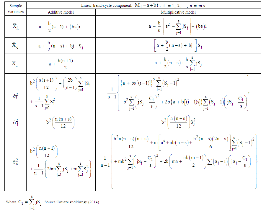 | Table 1. Summary of Row, Column and Overall Averages and Variances of Buys-Ballot for Additive and Multiplicative Models |
2.1. Row, Column and Overall Means and Variances of the Buys-Ballot table for the Mixed Model when trend-cycle Component is Linear
Following the way of [1], the row, column and overall means and variances were obtained for the multiplicative and the mixed models with the error terms. The summary of the row, column and overall means and variances for the mixed model, when trend cycle component is linear, is given in Table 2, while comparing them with those of the multiplicative model. As Table 2 shows, the row, column and overall means and variances are not the same for both mixed and multiplicative models. However, while the expected values of the row, column and overall means are the same for both multiplicative and mixed models, the expected values of the row, column and overall variances are not the same for the two models. Furthermore, the expected values of the row and overall variances involve sum of squares and cross-products of trend parameters and seasonal indices. The column variance, on the other hand, is for the mixed model, a constant multiple of the square of the seasonal effect and for the multiplicative model, the product of a quadratic function of j and the square of the seasonal effect. Therefore, to distinguish a series that admits the mixed model from one that admits the multiplicative model, an analyst only needs to look at the column variances  of the series in Buys-Ballot table. The appropriate test for choice between the mixed model and multiplicative model is, therefore, proposed based on the column variances.
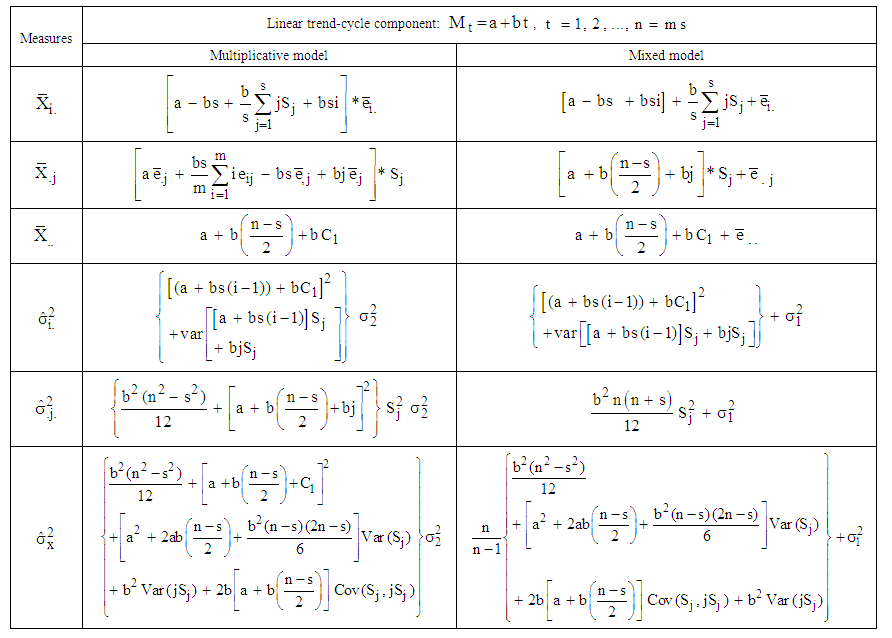 | Table 2. Summary of Row, Column and Overall Means and Variances of Buys-Ballot for Mixed and Multiplicative Models |
2.2. The Proposed Test for Choice between the Mixed and Multiplicative Models when Trend-cycle Component is Linear
As noted earlier, the column variance is, for the mixed model, a constant multiple of square of the seasonal effect only and for the multiplicative model, a quadratic function of the season j and square of the seasonal effect  . Therefore, the proposed test for choice between the Mixed and the Multiplicative models is based on the column variances.
 of the Buys-Ballot table. Hence, the null hypothesis to be tested is
 and the appropriate model is mixed, against the alternative
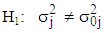 and the appropriate model is not mixed, where
 is the actual variance of the jth column.
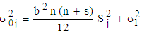 | (10) |
and  is the error variance, assumed equal to 1.Under the null hypothesis, [11] have shown that the statistic
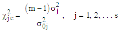 | (11) |
follows the chi-square distribution with  degrees of freedom and the sum;
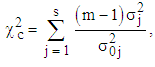 | (12) |
follows the chi-square distribution with  degrees of freedom, where m is the number of observations in each column and
  is the seasonal lag (number of columns). In proposing the test, we have assumed that (i) the underlying distribution of the variable,
  ,
, 
 under study is normal, (ii) the observations in each column,
  are independent and (iii) that the s-columns are independent.[11] also showed that under the null hypothesis, the interval
 contains the statistic (12) with
  degree of confidence.For the purpose of calculation of
  , both b and Sj are derivable from column mean
 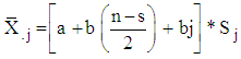 , rewritten as
 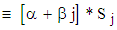 | (13) |
where, 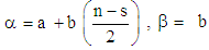 Estimates of
  are derivable from the regression of
  on j and estimates of
  is
is  | (14) |
where satisfies  as in (9). Limitations of the Proposed TestOne of the limitations of proposed test is the violation of some of the assumptions of Chi-square test. Neither the m observations within each group nor the s- groups are independent because the data under study is time series data.
3. Empirical Examples
In this section, we present some empirical examples to illustrate the applicability of the proposed test when the trending curve is linear. The empirical examples consist of simulated series from the mixed and multiplicative model. Results from simulations using mixed model are contained in Section 3.1. Section 3.2 presents results from simulations based on multiplicative model.
3.1. Simulations Results from Mixed Model
The first example is based on the 100 simulations of 120 observations each from 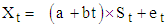 , with
  ,
,  ,
,  and
and  given in Table 3.
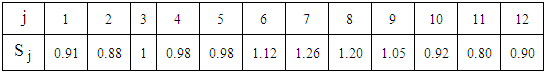 | Table 3. Seasonal  indices used in the simulation of series indices used in the simulation of series |
Each series has been arranged as monthly data (s = 12) for 10 years (m = 10). The column variances of the 100 simulations are contained in Appendix A. The proposed test statistic for choice between mixed and multiplicative models given in (11) requires the calculation of the Chi-square statistic and comparing it with the critical values,  ,
,  . Under the null hypothesis that the appropriate model is mixed, the calculated value of the statistic in (11) is expected to lie within the interval, otherwise, it will be concluded that the data does not admit mixed model. At 5% level of significance, the critical values are for
  degrees of freedom, equal to 2.7 and 19.0. For the proposed test statistic in (12), the decision rule is to reject the null hypothesis if the statistic in (12) lies outside the interval
  or do not rejected it otherwise. Again at 5% level of significance, the critical values are, for
  degrees of freedom, equal to 70.1 and 129.6.The calculated values of the statistic from the simulated series are contained in Table 4 When compared with the interval 70.1and 129.6, the calculated values of the statistic lie within the interval in 98 out of the 100 simulations. This indicates that the test is capable of identifying the model correctly 98 percent of the times. This expresses the level of confidence in the proposed test.
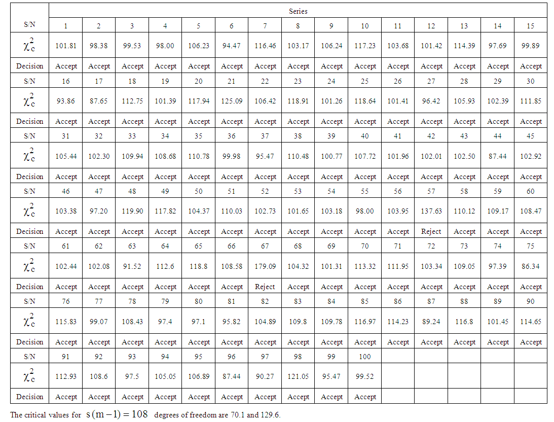 | Table 4. Calculated Chi-Square for Mixed Model |
3.2. Results from Simulations Using Multiplicative Model
The second example is based on the 100 simulations of 120 observations each from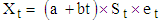 , with
  ,
,  ,
,  and
and  also given in Table 5 Each series of 120 observations has been arranged in a Buys-Ballot table with m = 10 rows and s = 12 columns. The column variances of the 100 simulations are contained in Appendix B while the calculated values of the test statistic are given in Table 5. As in section 4.2, the critical values at 5% level of significance and
  degrees of freedom are 2.7 and 19.0. Under the null hypothesis that the appropriate model is mixed, the calculated value of the statistic in (11) is expected to lie within the interval, otherwise, it will be concluded that the data does not admit the mixed model. When compared with the critical values, 97 out of 100 calculated values of the statistic from the simulated series given in Table 5 lie outside the interval, indicating that they do not admit the mixed model. In other words, the proposed test is capable of identifying the model correctly 98 percent of the time.
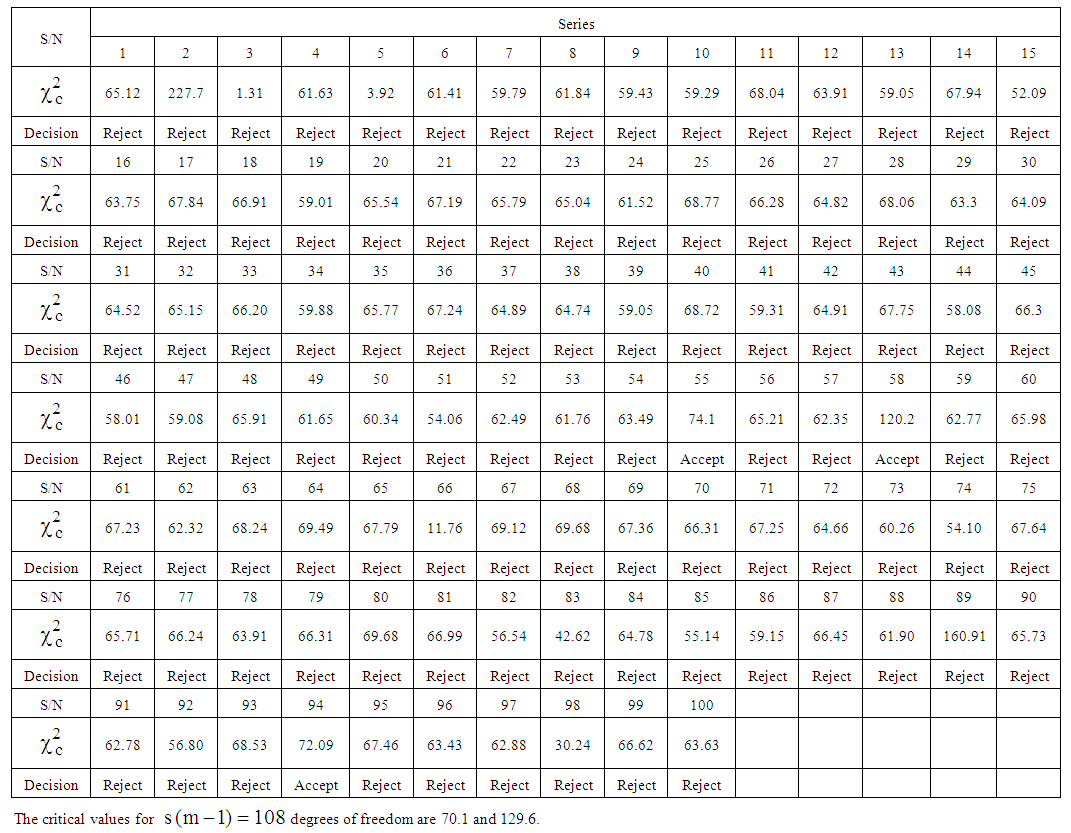 | Table 5. Calculated Chi-Square for Multiplicative Model |
4. Summary, Conclusions and Recommendations
This paper has discussed the procedure for distinguishing a series that admits the mixed model from one that admits multiplicative model in time series decomposition when the trend-cycle component is linear. If an analyst encounters a time series data, the first thing is to arrange it in Buys-Ballot table, calculate the column variances and apply any of the known tests for a constant variance. If the null hypothesis of constant variance is accepted, it indicates that the study series admits the additive model. When the null hypothesis is rejected the test proposed in this study provides a basis for choosing between mixed and multiplicative models. The proposed test is based on Chi-Square distribution. Although time series data does not satisfy all the assumptions of most common statistical tests, the Chi-Square test appears to be the most efficient among them. The proposed test is able to distinguish between the mixed and multiplicative models with a high degree of confidence and is hereby recommended.
References
| [1] | Iwueze, I. S. & Nwogu, E.C. (2014).Framework for choice of models and detection of seasonal effect in time series. Far East Journal of Theoretical Statistics 48(1), 45– 66. |
| [2] | Kendal, M. G. & Ord, J. K. (1990). Time Series (3rded.). Charles Griffin, London. |
| [3] | Chatfield, C. (2004). The analysis of time Series: An introduction. Chapman and Hall,/CRC Press, Boca Raton. |
| [4] | Puerto, J. & Rivera, M. P. (2001). Descriptive analysis of time series applied to housing prices in Spain, Management Mathematics for European Schools 94342 – CP – 2001 – DE – COMENIUS – C21. |
| [5] | Linde, P. (2005). Seasonal Adjustment, Statistics Denmark. www.dst.dk/median/konrover/13-forecasting-org/seasonal/001pdf. |
| [6] | Iwueze, I.S., Nwogu, E.C., Ohakwe, J. & AjaraoguJ.C. (2011). Uses of the Buys – Ballot table in time series analysis. Applied Mathematics Journal 2, 633 –645. |
| [7] | Iwueze, I. S. &Nwogu E.C. (2004). Buys-Ballot estimates for time series decomposition, Global Journal of Mathematics, 3(2), 83-98. |
| [8] | Wei, W. W. S (1989). Time series analysis: Univariate and multivariate methods, Addison-Wesley publishing Company Inc, Redwood City. |
| [9] | Iwueze, I. S. & Nwogu, E.C. (2005). Buys-Ballot estimates for exponential and s-shaped curves, for time series, Journal of the Nigerian Association of Mathematical Physics, 9, 357-366. |
| [10] | Iwueze, I. S. and Ohakwe, J. (2004). Buys-Ballot estimates when stochastic trend is quadratic. Journal of the Nigerian Association of Mathematical Physics, 8, 311-318. |
| [11] | Mood, A.M., Graybill, F.A. & Boss, S.C. (1974). Introduction to the theory of Statistics (3rd ed.). McGraw-Hill, New York. |

 Abstract
 Reference
 Full-Text PDF
 Full-text HTML