1. Introduction

Weather forecasting is mostly used to solve the system of complex equations. Weather forecasting is the application of technology and science to foresee the condition of atmosphere for a given position. Several of the live systems depend upon weather situations to make necessary modifications in their systems. Forecasting aid to take essential measures to prevent destruction to life and property to a great extent. Satellites, sensors and ground stations that are located surrounding of our planet, which have data of great quantity which send information on a daily basis and used the weather situation to foresee in the next day [1]. The weather forecasting is live forecasting where out-turn of the model may be required for everyday weather guide or weekly or monthly weather plans.

Time series analysis is widely used in weather data. Time series modeling is the procedure of forecasting using historical records. Time series analysis have been widely used in huge number of practical problems comprising modeling and forecasting economic time series and process. To estimate the time series data, we have used data mining techniques and also used patterns in parameters of weather data such as; wind direction, relative humidity and temperature. However, we only used temperature (low, high) and wind speed of weather forecasts. We need to keep them together for absolute forecast. All the data is collected from the meteorological department, Quetta city. Parameters of weather are as follows [2]:

1) Temperature: is an analysis of coldness and hotness in the air and is recorded in the Celsius (C⁰).

2) Wind speed: is related to convert in pressure of air at 1200 UTC (knots)”.

Sequential order is taken to measure the time series data within a certain time [3]. We have used Auto Regressive Integrated Moving Average (ARIMA) model in our study because the characteristics of streaming stationarity (Calculations do not depend on lag, mean, variance and covariance) [4]. The model is also called Box-Jenkins model, which is developed in 1976 [3].

Seasonal ARIMA (SARIMA) model is the extension of ARIMA model that is relevant of seasonal time series. Construction of SARIMA is considered as series of seasonal model [5]. There is relationship between ARIMA and SARIMA, in which the daily variation can be considered [6]. Weibull Distribution (WD) has been considered for expressing the wind speed variation. It represents various distribution characteristics when its parameter shape and scale are appropriately tuned. Therefore the Weibull model can be applied for modelling wind speed changes and forecasting future wind speed. Artificial Neural Network (ANN) is used in our paper for forecasting and analyzing the tendency and prediction of the data. ANN has the non-linear relationship between prediction and predictor, also able to general uncertainty of the function. That is similar to forecast the actual weather data and can be predicted large number of data. In this research Multi-Layer Perceptron (MLP) architecture is used. Back Propagation Neural Network (BPNN) is proposed to forecast the values of the parameter [7].

We studied the data to analyse the best model with least Akaike Information Criteria (AIC) value of ARIMA and the least Root Mean Square Error (RMSE) of the ANN to evaluate temperature and wind in the last five years. This research has benefits to select better methods amongst all, and develop a method for prediction to overcome the quantitative modeling forecasting. Data processing is used which is done by some software such as Minitab, MS excel, R software and NeuroSolutions software [8]. In this research, we used R software NeuroSolutions, MS excel and that has also facility to solve the problem of ARIMA. The objective of this study to forecast the future values of the parameters [9]. In this paper, the execution of ANN and ARIMA models is considered to decipher an instance of parameter including temperature and wind [8]. This paper is organized such as: Section 2 shows literature review and section 3 describes methodology. Computational results are shows in section 4. Future work and conclusion of this work are described in section 5.

2. Literature Review

Purnomo et al. emphasize models using ANN month’s rainfall data [7]. Murat. et al. used Box-Jenkins ARIMA, SARIMA and regression models on weather data to produce sensible forecast. Their experimental results show that monthly mean temperature surface of India vary [10]. Narvekar and Fargose used different techniques of ANN in which BPP Algorithm performs best prediction with minimal error [11]. Adebiyi et al. made comparison of ARIMA and ANN model on stock data. The empirical results obtained by the authors reveal the superiority of ANN models over ARIMA model [8]. Basheer et al. also compared ANN and classical Box-Jenkins models on Consumer price data of Yemen. The experimental results show ANN better predictive values than natural stochastic models [12].

Murat M., Krzyszczak J et al. found the forecasting of metrological materials which depicts the courses of future on the basis of previous time series model, and is beneficial for agro physical models [13,14]. El-Mallah E.S et al. interpreted the performance of quadratic ARIMA and linear ARIMA which make annual short-term forecasting of temperature [15]. Balyani Y et al. studied temperature of air-surface of monthly basis mean and used SARIMA model to forecast [16]. Hu proposed ADALINE system to forecast weather which is newly proposed applications of ANN in forecasting of weather [17].

Kaur, A et al used ANN to forecast temperature on an hourly basis, 24 hours ahead wind speed and relative humidity. The data is divided into four seasons. The experimental results show that Radial Basis Function Network (RBFN) is used to compare with MLP, Hopfield Network Model (HFN) and Elman Recurrent Neural Network (ERNN) [18]. Ch.Jyosthna Devi, developed an algorithm to forecast the temperature. The BPNN is used to fairly approximate the function of large class. Authors used a model which have real time data set with maximum and minimum normalization scale of the data between (0 to 1) then trained and tested the data by using BPNN. The experimental results are compared to validate and check model accuracy and least error [19]. Kamal, L., & Jafri, Y. Z used simulations of stochastic and forecasting models of hourly average wind speed. They found ARMA (p, q) which is appropriate for probability forecast and prediction intervals [20]. Mehrdad. et al used artificial neural network and stochastic models to forecast the monthly flow discharge of the Ghara-Aghaj River the results revealed that MLP and RNN had superior performance than ARIMA [21]. Kumar Abhishek et al. studies the applicability of ANN by constructing non-linear models for weather forecast, the researcher also compared the performance of established models using different transfer function, neurons and hidden layer to predict maximum temperature for 365 days [22]. Anosh Graham et al. used seasonal ARIMA model to forecast future rainfall and found that ARIMA model yield comparatively better forecast than the simple models [23]. Athraa Kadhem et al. used the wind speed data and apply WD model to predict the next day forecasting and the proposed model utilizes the ANN to predict the wind speed data. The results indicate that the proposed ANN model is capable of depicting the fluctuating wind speed during different seasons of the year at different locations [24].

3. Methodology

Methodology adopted for conducting this study includes stochastic models and ANN with R software and Neuro solution Version 7.

3.1. Statistical Models

Box-Jenkins is considered in this research followed by [25]. This model is dependent on different steps:

• Appropriate model is identified from the ARIMA model family.

• Model of estimation.

• To verify the model we check the suitability of under-study-series, when that is not suitable then we return back to the first step, if not then forward to the next step.

• Model that is selected is used for prediction.

3.1.1. ARIMA

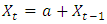
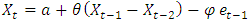
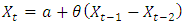
These are models used for forecasting a stationary time series by one and more times differencing. An ARIMA model generally denoted as ARIMA (p, d and q) where p is the order of auto-regressive, d is the degree of differencing and q is the number of lagged forecast.

In term of X the general forecasting equation is

Here auto regressive parameter and moving average parameters are defined.

3.1.2. SARIMA

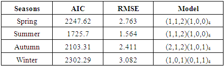
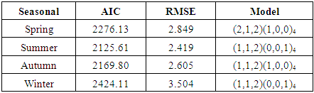
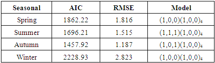
ARIMA is the extension form of these models and is used for seasonal time series. It is used for forecasting of time series with univariate data having seasonality and trends. The SARIMA (p, d, q) (P, D, Q) m process as SARIMA (p, d, q) (P, D, Q) m is given by

In SARIMA we analyze the long term trend and seasonal effect. SARIMA is based on ARIMA models to change time series data.

3.2. Artificial Neural Network

Neural Network (NN) is important domain of Artificial Intelligence (AI) that is used in complex and modern applications of modern science, which is as follows: industry of robotic systems, systems of decision support, automated control systems, prediction and identification systems.

ANN is a tool of effective forecasting [26] and consist of algorithm, which mimic the feature of human being brain that explore and generate basic knowledge by research [27]. ANN contains different components, which need to be carefully calculated because it effects the performance of forecasting method. ANN define some different elements such as Machine Learning Algorithm and architecture structure. The architecture is defined by different number of layers, number of neurons in all the layers and the rules that determine the architecture. Feed-Forward Back Propagation Neural Network (FFBPNN) is one of the type of neural network which is mostly used for forecasting. FFBPNN algorithm is mostly used as learning algorithm which updates the weights dependence on the variation in to the output value of the NN and desired real value. Figure 1, Shows ANN model the given input layer shows the action which is fed in to next layer until the output layer.

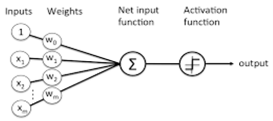Figure 1. Single layer Neural Network

3.3. Weibull Distribution

We calculated the Weibull probability density functions. There are serval methods [28] for determining the Weibull parameters c and k using Justus relations for c and k, i.e. the scale parameter and the shape parameter we obtained the following.

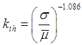And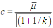

4. Computational Results

The proposed method is provided in this section by results that are experimented. First of all we described data description that are used in the experimental results. The results are presented by using the Box-Jenkins method of statistics and then ANN results are compared and analyzed. The error measurements are forecasted by the use of estimating the method for forecasting. These error measurements that are used such as: RMSE for ANN and AIC value for ARIMA and SARIMA models.

4.1. Data Description

For conducting this study we obtained daily recorded data of five years period (2012-16) from Meteorological Department, Quetta. The obtained record includes daily maximum, minimum temperature and wind speed observations.

4.2. Prediction Using Statistical Model (Box-Jenkins)

The R software is used as statistical program, which identify the suitable model for data by using ARIMA model for AIC value, Auto-Correlation Function (ACF) and Partial Autocorrelation (PACF). Table 1, 2 and 3 show all results of Temperature Maximum, Minimum and wind speed respectively.

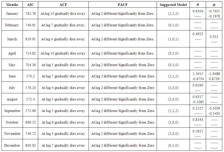Table 1. ARIMA modelling for maximum temperature and identification of the model

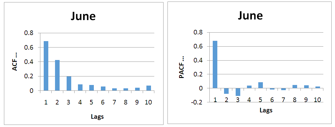Figure 2. (a) Shows autocorrelation function verses lag by ARIMA model. (b) Shows partial-autocorrelation function verses lag by ARIMA model

4.2.1. Prediction Equations of Maximum Temperature

ARIMA (0, 1, 0) is the model that is used for the months of February, April, May and December. ARIMA (1, 0, 0) for July, October and November. ARIMA (1, 1, 2) for January and September. ARIMA (2, 1, 2) for June. ARIMA (2, 0, 0) for August. And ARIMA (1, 0, 1) for March.

• The Non-Seasonal ARIMA equations are as follows

ARIMA (0, 1, 0)

ARIMA (1, 0, 0)

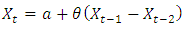ARIMA (1, 1, 2)

ARIMA (2, 1, 2)

ARIMA (2, 0, 0)

ARIMA (1, 0, 1)

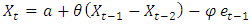Respectively where is constant, is the error at period (t-1),

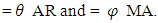
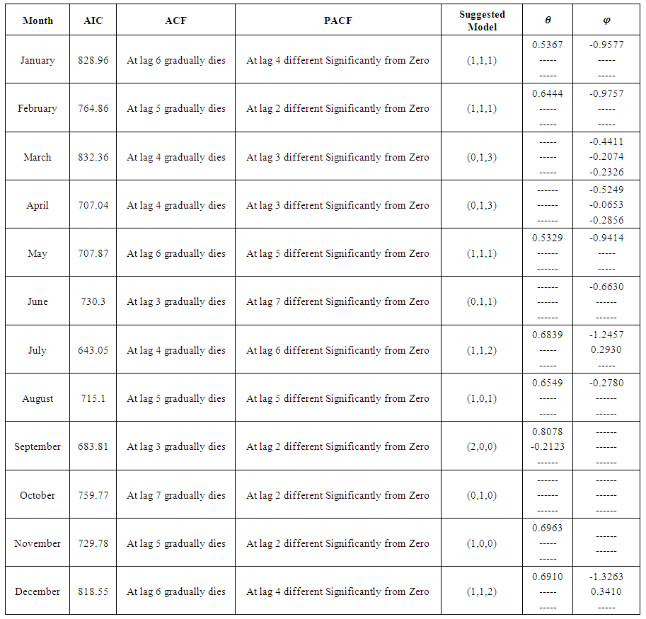Table 2. ARIMA modelling for minimum temperature and identification of the model

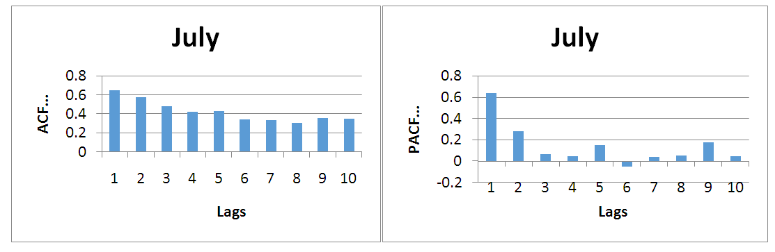Figure 3. (a) Shows autocorrelation function verses lag by ARIMA model. (b) Shows partial-autocorrelation function verses lag by ARIMA model

4.2.2. Prediction Equations of Minimum Temperature

ARIMA (1, 1, 1) model is taken for the months of January, February and May. ARIMA (0, 1, 3) March, April. ARIMA (1, 1, 2) for July, December. ARIMA (0, 1, 1) for June. ARIMA (1, 0, 1) for August. ARIMA (2, 0, 0) for September. ARIMA (0, 1, 0) for October. And ARIMA (1, 0, 0) for November.

• The Non-Seasonal ARIMA equations are as follows

ARIMA (1, 1, 1)

ARIMA (0, 1, 3)

ARIMA (1, 1, 2)

ARIMA (0, 1, 1)

ARIMA (1, 0, 1)

ARIMA (2, 0, 0)

ARIMA (0, 1, 0)

ARIMA (1, 0, 0)

Respectively where is constant, is the error at period (t-1),

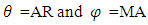
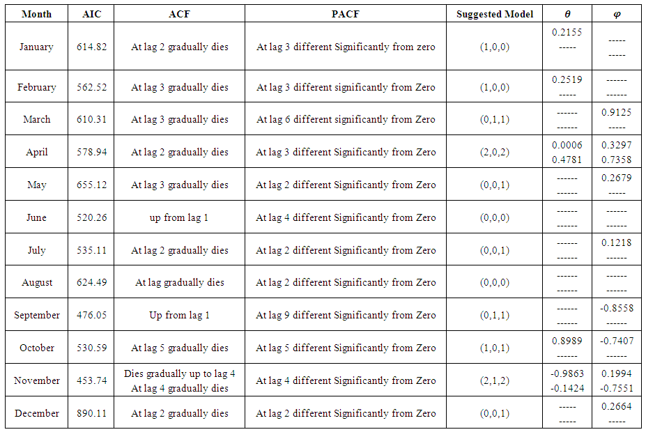Table 3. ARIMA modelling for wind speed and identification of the model

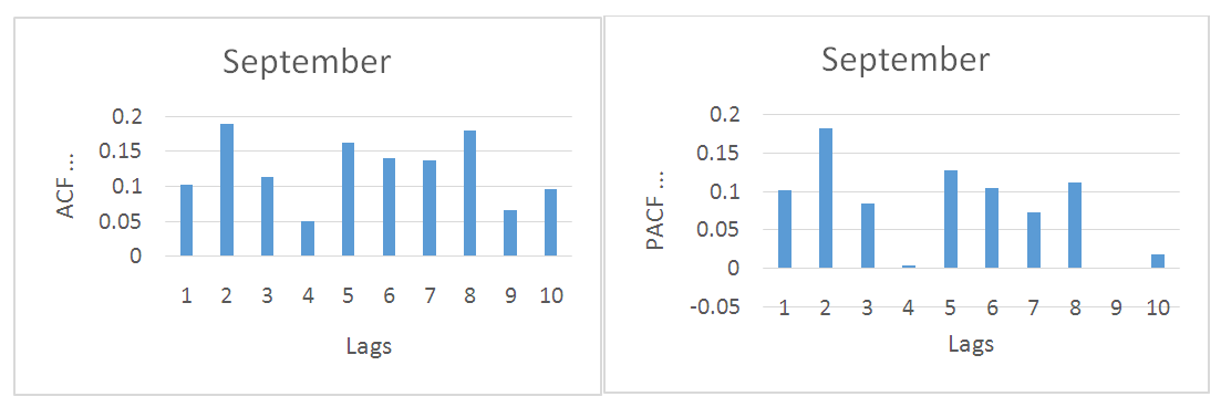Figure 4. (a) Shows autocorrelation function verses lag by ARIMA model. (b) Shows partial-autocorrelation function verses lag by ARIMA model

4.2.3. Prediction Equations of Wind Speed

ARIMA (1, 0, 0) for January and February. ARIMA (0, 1, 1) for March and September. ARIMA (0, 1, 1) May, July, December. ARIMA (2, 0, 2) for April. ARIMA (0, 0, 0) for June and August. ARIMA (1, 0, 1) for October. ARIMA (2, 1, 2) for November.

• The Non-Seasonal ARIMA equations are as follows

ARIMA (1, 0, 0)

ARIMA (0, 1, 1)

ARIMA (0, 0, 1)

ARIMA (2, 0, 2)

ARIMA (1, 0, 1)

ARIMA (2, 1, 2)

Respectively Where is constant, is the error at period (t-1),

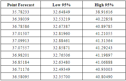
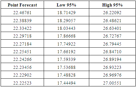
The model that is identified for the data is ARIMA (2,1,2), (1,1,2) and (0,1,1). These results are achieved in approximated parameters test of significant and also achieved analysis of residential test (in other words, it is achieved for this model in test of diagnostic). Table 4. Represents the best results among the all parameters with least AIC value.

Table 4. Best Models of ARIMA that shows the suitability of time series data

Figure 5 the graphs of the forecasting on under study data by using Box-Jenkins model in which the recorded data is shows in black curve and forecasted data is shows in blue curve.

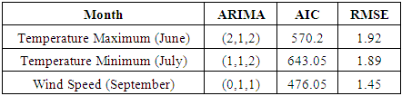
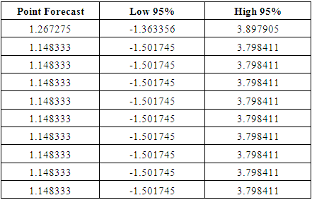
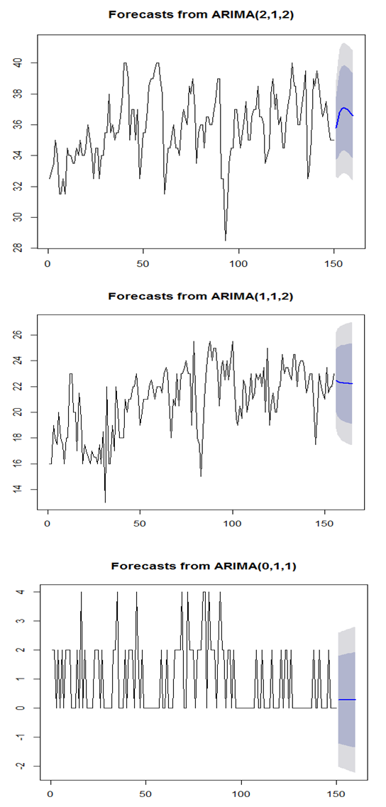Figure 5. Prediction using Statistical Models (Box-Jenkins)

Table 5 to 7 show the predicted values of maximum temperature, minimum temperature and wind speed having 95% C.I of Lower and Upper limits. While Tables 8 to 10 defines AIC, RMSE values and seasonal SARIMA classification on the basis of all four seasons of Quetta from spring to winter having their corresponding months for all the three selected parameters.

Table 5. Shows the Forecasting Temperature Maximum values of ARIMA Model (June)

Table 6. Shows the Forecasting Temperature Minimum values of ARIMA Model (July)

Table 7. Shows the Forecasting Wind Speed values of ARIMA Model (September)

Table 8. SARIMA modelling for maximum temperature and identification of the model

Table 9. SARIMA modelling for minimum temperature and identification of the model

Table 10. SARIMA modelling for wind speed and identification of the model

4.3. Forecasting Using ANN Model

The accomplishment in execution of Neural Networks relies upon the comprehension and suitable decision variable of input. If there should arise an occurrence of accomplishing an anticipating with respect to the time series, the Neural Network will have one yield provided the determined esteem and the data sources might be spoken to through estimations of the factors investigated at various past minutes. Table 11 to 13 shows the values of ANN in the way that system presents the input layer as 20, 50 and 80 neurons having single layer of output with Training =45%, cross validation =15%, Testing =40%, Layer =1, Epoch =150 and bold values represent best results. The outcomes of RMSE utilizing this technique are in table 14 and actual and predicted values are shown in Figure 6.

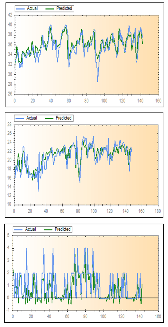Figure 6. (a) Shows the neural network prediction of temperature maximum data and one hidden layer. (b) Shows the neural network prediction modeling of temperature minimum data and one hidden layer. (c) Shows the neural network prediction modeling of wind speed data and one hidden layer

4.4. Comparative Study

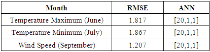
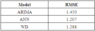
The Box-Jenkins model used for time series prediction on weather data assumes that there is a linear relationship between input and output. NN approximate the non-linear functions and have been successfully used for that future forecasting. Table 14 shows the proposed NN models, for June, July and September [20,1,1] perform better than classical Box-Jenkins models (2, 1, 2), (1, 1, 2) and (0, 1, 1) for the months of June, July and September. This can be shown in table 4. Using forecast error measurement like RMSE. We also used WD on wind data from January 2012 to December 2016. The table 15 shows the comparative study of ARIMA, ANN and WD. Figure 7 shows the predicted and actual values for the month of September. The comparison confirms the superiority of the proposed ANN to ARIMA and WD.

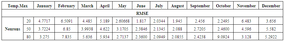Table 11. ANN results of Maximum Temperature

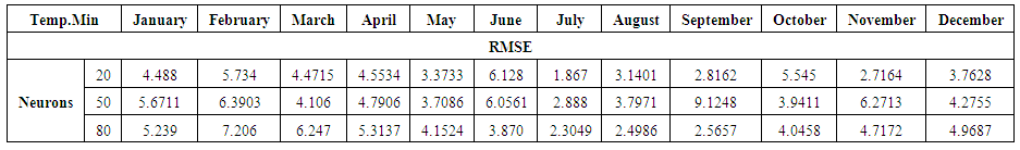Table 12. ANN Results for Minimum Temperature

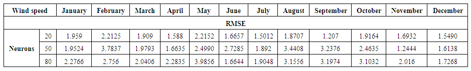Table 13. ANN Results for Wind Speed

Table 14. Results for the proposed ANN method

Table 15. Results of WD for the month of September

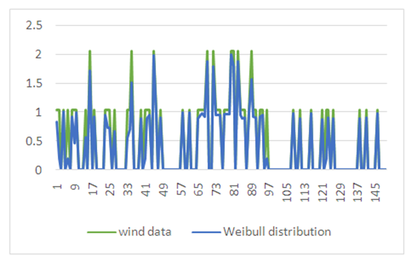Figure 7. Predicted and actual values for the month of September

5. Conclusions

In this paper two methods for model identification and forecasting are used, one is based on stochastic models like ARIMA and SARIMA for short and long term variations on weather data, respectively and the other proposed model using ANN. Comparison between the statistical model and proposed ANN model showed that the proposed model gave lower error and higher accuracy of time series data. We also apply Weibull distribution on wind data. Table 15 shows the comparison of ARIMA, NN and WD. Comparison is made on the basis of RMSE. NN is best amongst three.