1. Introduction

Regression analysis is a statistical method widely used in many fields such as Statistics, economics, technology, social sciences and finance. A linear regression model is constructed to describe the relationship between the dependent variable and one or several independent variables. All procedures used and conclusions drawn in a regression analysis depend on assumptions of a regression model. The most used model is the classic linear regression model and the most used method for estimating classic model parameters is the Ordinary Least Squares (OLS).

The linear regression model

(1)

The matrix form can be expressed as

(2)

where

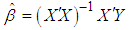
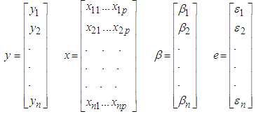Normal equation in matrix form. Given n for one predictor variable (say )

(3)

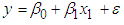
The sample estimate of can be written as

(4)

This is expressed as

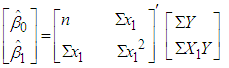
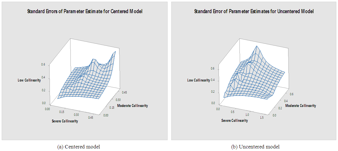
Under the classic assumptions, the OLS method has some attractive statistical properties that have made it one of the most powerful and popular methods of regression analysis. However, OLS is not appropriate if the explanatory variables exhibit strong pair wise and/or simultaneous correlation (multicollinearity), causing the design matrix to become non-orthogonal or worse, ill-conditioned. Once the design matrix is ill-conditioned, the least squares estimates are seriously affected, e.g., instability of parameter estimates, reversal of expected signs of the coefficients, masking of the true behavior the linear model being explored, etc. Furthermore, it reveals that small change in the data may lead to large differences in regression coefficients, and causes a loss in power and makes interpretation more difficult since there is a lot of common variation in the variables (Vasu and Elmore 1975; Belsley 1976; Stewart 1987; Dohoo et al., 1996; Tu et al., 2005).

The problem of multicollinearity commonly exists among economic indicators that are influenced by similar policies that lead their simultaneous movement along similar directions.

Whether co-integration exists or not among the predictors, simultaneous drifting away in some directions especially among time series that exhibit non-stationary behavior is common.

There are many solutions proposed in the literature to address this problem. Among them are Dropping of variables (Carnes and Slade, 1988), the general shrinkage estimators (Hoerl and Kennard 1980; McDonald and Galarncau, 1975; George and Oman, 1996; McDonald, 1980), principal component regression (Butler and Denham, 2000), then centering (Aiken & West 1991, Cronbach 1987, Irwin & McClelland 2001). However, there is a growing debate on whether or not to involve centering as a solution for a collinear regression. It has been argued that the source of any discrepancies among statistical findings based on regression analyses in absence of centering is not mysterious; they can always be explained and resolved. Various researchers including Aiken and West (1991); Cronbach (1987), and Jaccard, Wan & Turrisi (1990); Irwin & McClelland, (2001); and Smith & Sasaki, (1979) recommend mean centering the variables x₁ and x₂ as an approach to alleviating collinearity related concerns. Aiken, West and others further recommend that one centre only in the presence of interactions. Centering aids interpretation and reduces the potential for multicollinearity (Aiken and West 1991). It is therefore a strategy to prevent errors in statistical inference. Aiken and West (1991) also imply that mean-centering reduces the covariance between the linear and interaction terms, thereby increasing the determinant of X’X. This viewpoint that collinearity can be eliminated by centering the variables, thereby reducing the correlations between the simple effects and their multiplicative interaction terms is echoed by Irwin and McClelland (2001, p. 109). Centering is recommended in order to eliminate collinearities which are due to the origins of the predictor variables and it can often provide computational benefits when small storage or low precision prevail (Marquardt and Snee, 1975).

However, in contrast to Cronbach’s injunction, other authors (Glantz & Slinker, 2001; Kromrey & Foster-Johnson, 1998; Belsley, 1984; Echambadi & Hess 2007) take the stand that centering doesn’t usually change the statistical results, is necessary only in certain circumstances, and can thus easily be. Few authors like Hocking (1984), Snee (1983), Belsley (1984b), have attempted to address this problem but did not extend to the polynomial regression especially the two predictor variables. The problem of centering is therefore an issue which is still not completely resolved. In this article, we clarify the issues and reconcile the discrepancy. Therefore the aim of this paper is to compare the statistical estimates of a centered mode in a second order regression model at various degrees of collinearity for two predictor variables (X₁&X₂) in a linear component, quadratic component and interaction (cross product).

The rest of the paper is mapped out as follows: Section 2 presents related literature and theoretical perspective of polynomial regression. Section 3 is the materials and methods of the paper, following interpretation of the empirical result, section 4 is the conclusion of the paper.

2. Polynomial Regression

In Statistics polynomial regression is a form of linear regression in which the relationship between the independent variable x and the dependent variable y is modeled as an n^th degree polynomial. Polynomial regression fits a nonlinear relationship between the value of x and the corresponding conditional mean of y, denoted E(y/x). In general, we can model the expected value of y as an n^th degree polynomial. The polynomial regression model may contain one, two, or more than two predictor variables. Each predictor variable may be present in various powers.

(5)

Further, each predictor variable may be present in various powers. We begin by considering a polynomial regression model with one predictor variable raised to the first and second power

(6)

where

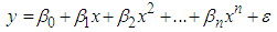
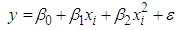
This polynomial model is called a second-order with one predictor variable because the single predictor variable is expressed in the model to the first and second powers. The predictor variable is centered – that is, expressed as a deviation around its mean and that the i^th centered observation is denoted by.

The two predictor variables of second order is given by

(7)

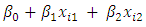where represents the linear component, = quadratic component and which is the cross product or interaction component.

The above is a second-order model with two predictor variables. The response function is:

(8)

Centering is defined as subtracting the mean (a constant) from each score, X, yielding a centered score. It is therefore an important step when testing interaction effects in multiple regression to obtain a meaningful interpretation of results. Centering the variables places the intercept at the means of all the variables. A regression equation with an intercept is often misunderstood in the context of multicollinearity. The intercept is an estimate of the response at the origin where all independent variables are zero, thus inclusion of the intercept in the study of collinearity is not of much interest. When variables have been centered, the intercept has no effect on the collinearity of the other variables (Belsley, Kuh, and Welsch, 1980). Centering is also consistent with the computation of the variance inflation factor (VIF) and therefore it is suggested that VIF be computed only after first centering variables (Freund, Littell, and Creighton, 2003).

Ostertagová, (2012) describe how polynomial regression model is useful when there is reason to believe that the relationship between two variables is curvilinear, and illustrated using data from a drilling-hole in the engineering field. Michael et al (2005) describes the reason for centering predictor variable in the polynomial regression model is that X and X² will often be highly correlated, and recommended centering as a means of reducing the multicollinearity. They observed that after the regression model has been fitted, the fitted values and residuals for the regression function in terms of X are exactly the same as the regression function in terms of the centered values of x. Also they stated that the estimated standard deviations of the regression coefficients in terms of the centered variables x do not apply to the regression coefficient in terms of the original variables of X. A number of scholars have considered issues related to mean centering with regard to the inclusion of product terms in a multiple regression model to test for moderators (Iacobucci et al., 2016). They noted that mean centering variables does not change the nature of the relationships between any variable in the set that does not include the product term.

Aitken and West (1991) encourages centering only in the presence of interactions while David and Richard (2011) in their work describes the term centering on mean as subtracting the mean value from an independent variable, in their work they noted that the interaction coefficient does not change from the non centered model to the centered model. Kramer and Bassay (2005), in a study on “centering in regression analysis: a strategy to prevent errors in statistical inference”, noted that non centered data in regression analysis, often leads to inconsistent and misleading results. Also that centering does not change the predicted values when predictor values are perfectly correlated except in the case of multicollinearity which are usually associated with models with interaction or a higher order term such as X². McClelland et. al. (2016) in their critical research verified the irrelevance of multicollinearity in the model with moderator variables. While Kaur (2017) observed that centering only helps multicollinearity disappear and doesn’t quite improve the regression model as such.

3. Materials and Methods

To show the effect of mean centering on an ill-conditioned regression model, we ran a Monte Carlo simulation study using SAS 9.0 version. We begin by multiplying each of the selected variable with 0.5 in order to make the variables uniform.

U= ranuni (start)

X₁=U+rannor (start)*0.5

X₂=U+rannor (start)*0.5

Y=1+X₁+X₂+rannor (start)

That is, we set ρX₁, Y=ρX₂, Y= 0.5 to represent modest sized effects of two predictors on the dependent variable, and varied the extent of multicollinearity, ρX₁, X₂ from 0.1 to 0.9. To achieve the objective of varying collinearity, we perturb the random error μ by multiplying it with values (i.e. 0, 1, 2, 3, 4, 5, 6, 7, 8, 9, 15, 30). This generates different values of the correlation coefficient between the two explanatory variables as shown in table 1.

Table 1. Table of values of correlation

Three different scenarios are considered from the above table 1, which have different correlation structures (i.e. low, moderate and severe) among the variables. Starting with the simplest case which assumes that two variables are uncorrelated or have minimal correlation with each other in a multivariable model. In this bivariate collinearity scenario, we investigate the effect of bias in estimates of related regressor coefficients due to the variation in the degree of collinearity between the centered and uncentered models. For the next group, we extend the first scenario by allowing some degree of collinearity among the variables (moderate collinearity). And in the last group, which is the case of severe collinearity where the degree of correlation between the variables is very strong. In each case, three components were captured and they include: (1) linear component, (2) quadratic form of a variable and (3) interaction of two variables. To evaluate the sample size variation on precision of estimation, for each level of ρX₁X₂, we generated a random sample of size N = 50, 100, 200, 500 and 1000 size. We computed a product score, X₁X₂. We ran a regression using the main effects and interaction, X₁, X₂, and X₁X₂ to predict Y. We obtained the β estimates, their standard errors, and the p-values representing their significance tests. We also took the same generated variables and mean centered X₁ and X₂. We computed the new product score, ran another regression, and obtained the new βs, standard errors, and p-values.

Case 1: Minimal Collinearity among the explanatory variables

This scenario assumes little or no correlation between the explanatory variables. Here we noticed that for linear component, the regression coefficients were higher in the centered model than the uncentered model. This is an indication that greater multicollinearity dampens the estimate of β. Since the standard error of the coefficient (SE Coef) indicates the precision of the coefficient estimates, the table shows that the centered model has more reliable estimates than the uncentered for linear component. By comparison, mean centering reduces standard errors and thus benefits p-values and the likelihood of finding β₁ or β₂ significant. This is unlike the case of quadratic and interaction term, both the mean-centered and the uncentered models for quadratic and interaction term provided an identical fit to the data. As expected, the coefficients of the interaction, the standard errors, and the t-statistics obtained from both the models are identical. A point that may confuse some researchers in this regard is that t-statistics for individual regressors may change when data are mean-centered. This does not occur for the quadratic and interaction term. As noted by Aiken and West (1991) and shown here, the coefficient and the standard error for the interaction term, and hence the significance of this term, will be identical with or without mean-centering. However, t-statistics may change for the linear terms as a result of shifting the interpretation of the effect. In a regression without mean-centering, the coefficients represent simple effects of the exogenous variables, i.e., the effects of each variable when the other variables are at zero. When data are mean-centered, the coefficients represent main effects of these variables, i.e., the effects of each variable when the other variables are at their mean values.

Table 2. Centered and Uncentered models with low collinearity

Case 2: Moderate Collinearity among the variables

In this case, we considered moderate collinearity between X₁ and X₂ variables. As shown in the table 3, here again the same scenario repeated itself for linear component in terms of regression coefficient and standard error but for the quadratic and interaction components were quite different. An examination of the variance inflation factor under moderate collinearity from Table 3 reveals that the Variance inflation factor (VIF) of the centered model indicated absence of collinearity (VIF < 10) in all the three components considered while for uncentered model, collinearity was present in all the components (i.e VIF >10). This may be an indication that mean centering helps to ameliorate collinearity problems in quadratic and interaction components judging by VIF < 10.

Table 3. Centered and Uncentered models with moderate collinearity

Case 3: Severe Collinearity among variables

This is a scenario where there is a very strong correlation between X₁ and X₂ variables. Table 4 indicates again that the standard error of centered model were lower than that of uncentered model for linear components but for quadratic and interaction components, the standard errors in both models were relatively the same. The VIF shows absence of collinearity in linear component judging with the rule of thumb (VIF < 10) but there was presence of collinearity quadratic and interaction components in the centered model. The uncentered models indicated that there is presence of collinearity in all the three components. It is interesting to note that the VIF of uncentered model is more than ten times VIF in centered model especially for quadratic and interaction components. Our findings here show that centering model helps to reduce collinearity problem. It should be pointed out that in using centered care must be taken on the degree of collinearity.

Table 4. Centered and Uncentered models with severe collinearity

The response of the centered and uncentered models was graphically represented by 3D response surface generated by the three cases (i.e. minimal collinearity, moderate collinearity and severe collinearity). Figures 1 and 2 depict the nature of how mean centering enhances a regression analysis. Figure 1 described the response of centered and uncentered models to multicollinearity using variance inflation factor (VIF). It may be also observed that with low collinearity, the centered model experienced VIF between 0 and 1.16 while the uncentered model responded to VIF between 0 and 4.20. However, with moderate collinearity VIF slightly increased further but was still less than 3 (VIF < 3) an indication of absence of collinearity. For the uncentered model, it was a different scenario entirely. The increase in VIF was very pronounced. Little wonder while the bumps on the graph with the uncentered model. When the collinearity was severe, the VIF of both the centered and the uncentered models were on the increase. As can be seen on the graph, a slight bump was experienced by the centered model unlike the case of the uncentered model which showed number of bumps.

Figure 1. Three-dimensional Relationship of linear, quadratic and interaction response to VIF in low-collinear, moderately collinear and severely collinear variables between centered and uncentered models

The effect of standard error on both centered and uncentered model was also represented in figure 2. With minimal collinearity, both models showed a negligible increase in standard error of estimates. For moderate collinearity, again, for centered model, the standard error becomes inflated with severe collinearity while for uncentered model; the standard error is inflated in all the three cases (minimal collinearity, moderate collinearity and severe collinearity). Surprisingly the direction of the peak among the standard errors varied in both models. This may be as a result of the lower standard errors of linear component in the centered model than that of uncentered model. While the standard error of the quadratic and interaction terms of the uncentered model were lower than that of the centered model.

Figure 2. Three-dimensional Relationship of linear, quadratic and interaction response to standard error in low-collinear, moderately collinear and severely collinear variables between centered and uncentered models

4. Conclusions

In this analysis, we focused on how three components (linear, quadratic and interaction) behave in centered and uncentered models to an ill conditioned regression using different collinearity structure (low, moderate and severe). A simulation study considering regression model with linear, quadratic and interaction components for centered and uncentered models was established. The result showed that the linear effect is significant in both the uncentered and mean-centered models for all the three considered collinearity structures, whereas quadratic and interaction effect were insignificant. Also, when there is a meaningful interaction among the variables, the linear effect will not equal the quadratic and interaction effect. It is worth to note that even the improvement offered by mean centering has its limits. When correlations is very strong, results begin to be affected even if the variables have been mean centered. The author believes that centering alleviates muticollinearity problem but it necessary to consider the degree of collinearity among the explanatory variables before using mean centering. For severe collinearity, use of centering should be discouraged especially for quadratic and interaction components.