Hüseyin Ünözkan1, Mehmet Yilmaz2
1Ankara University, Graduate School of Natural and Applied Science, Department of Statistics, Turkey
2Ankara University, Science Faculty, Department of Statistics, Turkey
Correspondence to: Hüseyin Ünözkan, Ankara University, Graduate School of Natural and Applied Science, Department of Statistics, Turkey.
| Email: |  |
Copyright © 2019 The Author(s). Published by Scientific & Academic Publishing.
This work is licensed under the Creative Commons Attribution International License (CC BY).
http://creativecommons.org/licenses/by/4.0/

Abstract
Nowadays, one of the aim of statistical studies is to provide the future with the models which are easily accessible and simple. Therefore, more suitable distributions are needed to model the data. In this study, a new distribution is generated with exponential marginals Farlie-Gumbel-Morgenstern distribution. Specifications and characteristics of this new distribution are studied. The structure of the proposed distribution is discussed statistically and the parameter estimation for the new distribution is made by known methods. In addition, reliability analysis has performed. Due to the shape and flexibility of the proposed distribution, it is thought to be an alternative to distributions which are used for modeling flow data. Efficiency on the statistical modeling of the new distribution can be detected by using flow data sets in literature. Furthermore, Terme and Sefaatli Creeks' flow-data obtained from Turkish State Water Affairs Directorate are used to model. It is concluded that this new distribution offers a model that can be used effectively in stream flows.
Keywords:
Falie-Gumbel-Morgenstern Distribution, Copula, Reliability Analysis, Generating Distribution, Exponential Distribution
Cite this paper: Hüseyin Ünözkan, Mehmet Yilmaz, A New Method for Generating Distributions: An Application to Flow Data, International Journal of Statistics and Applications, Vol. 9 No. 3, 2019, pp. 92-99. doi: 10.5923/j.statistics.20190903.04.
1. Introduction
Global warming has effected nearly every water sources. For estimating behavior of streams, modeling and analyzing flows has vital importance. In the world, the population rate is rising rapidly, which makes pure water resources more important. For some decades, researchers have studied in streams for estimating drought and flood. Till now, they have used some most known distributions for modeling streams statistically. After modeling, they have analyzed behavior of streams easily. Some stream statistics was described as magnitude, variability and flow extremes. Mean flow is the fundamental statistics of flow record. It is usually expressed as flow in m3/s. In order to measure the variability, it is the most common method to obtain the distribution of monthly average flows [3].Therefore, we can use the mean of annual flows, mean of the lowest month flows, and rivers' total flows to model their behavior. For low flows, Generalized Extreme Value distribution, Pearson Type III and Generalized Logistic distributions are commonly used. Sometimes these distributions can be used with more parameters than their original structure. A fourth distribution, the Generalized Pareto, was also offered [11]. In literature, we can find some transmutations for these distributions to better match streams flow data [4]. [11] shows which distributions are needed to analyze flow data, and in particular to analyze minimum values. We can estimate the behavior of the stream with mean flows, such that this can be important for living beings in the district of this stream.The frequency of floods was analyzed in [7] by hydrological functions through extremes and they used the same statistical distributions in [11]. In this paper, we suggest a new distribution for analyzing every kinds of stream data which are using for describing river behaviors. Through the paper, this proposed distribution is called as “CFGMWEM”. CFGMWEM presents good results especially in modeling low flows. In our presentation, we have first introduced CFGMWEM. After this we have shown new distribution's properties, and important characteristics. Finally, we have compared CFGMWEM with most known hydrologic statistical functions via data which were used in literature and new data obtained from Turkey rivers.
2. Materials and Methods [New Distribution (CFGMWEM)]
In recent years, during the measuring process of flows, mostly logical systems have been used. While measuring these values, logical machines obtain observation only if the flow level is higher than the lowest measuring point of them. According to this approach for fertile measurement, the heaviness of stream has to be more than a fixed point. The aim of this study is to develop a statistical model about the flow data which is observed during this real measurement process. In order to realize this, it is necessary to obtain a successful statistical model and this requires the use of an important theorem.Theorem (Sklar’s Theorem) Let  be a joint cumulative distribution function and
  and
and  is marginals, then there is a copula function
  in
in  for every
  and
and  [9].
[9].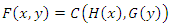 Farlie-Gumbel-Morgenstren (FGM) copula with marginals
  and
and  can be written as below [6].
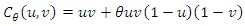 Hence, Two dimensional Bivariate FGM distribution with marginals
  and
and  is as follows.
 Probability density function of this distribution is as below.
 Under
Under  condition,
  has a conditional probability density function as follows.
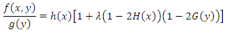 Under
Under  condition,
  has a conditional distribution as below.
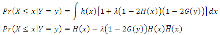 Under
Under  condition probability of
  is
is provided. Considering the models related to natural events, exponential distribution has a wide range of usability. Because of simple statistical structure and memoryless property exponential distribution has been used widely. Suppose that
  Then we have
 We know from the literature that the transmuted distribution with baseline
  is
is  . Here,
  is the failure distribution of the two-component parallel system (with identical and independent) namely, represented as
  In the light of this idea,
  can be also rewritten as the form of
  where
where  represents a failure distribution of 3 out of 2 system with independent and identical component. Thus, we have a different form of transmuted distribution. Hence when baseline distribution is assumed to be exponential we have the following special form of distribution.
 | (1) |
Probability density function of CFGMWEM is as below.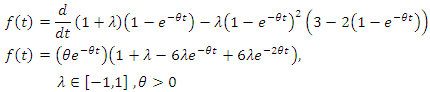 | (2) |
Some shapes of probability density function are as below. In Fig. 1 and Fig. 2 
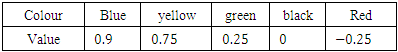
Table 1. Values of
 parameter matching by colour in Fig. 1 parameter matching by colour in Fig. 1
 |
| |
|
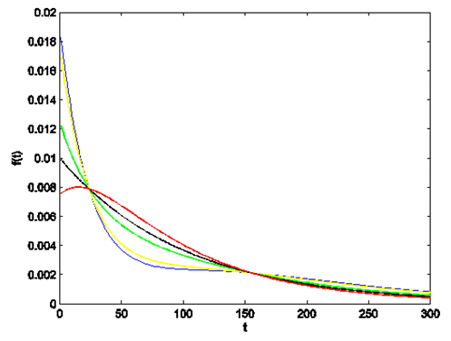 | Figure 1. Plots of probability density function |
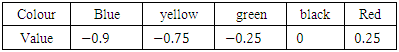
Table 2. Values of
 parameter matching by colour in Fig. 2 parameter matching by colour in Fig. 2
 |
| |
|
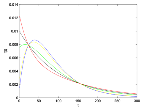 | Figure 2. Plots of probability density function |
Survival function of CFGMWEM is as follows;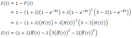 Hazard rate function of CFGMWEM is as below.
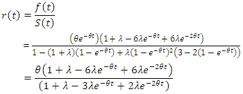 If we want to calculate the risk of the starting point;
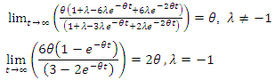
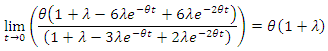 We reach that in the long term risk, there are two diffrent results according to the parameter
 Some shapes of hazard rate function are as below. In Fig. 3 and Fig. 4
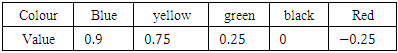
Table 3. Values of
 parameter matching by colour in Fig. 3 parameter matching by colour in Fig. 3
 |
| |
|
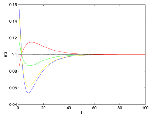 | Figure 3. Plots of hazard rate function |
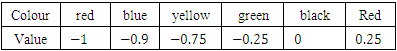
Table 4. Values of
 parameter matching by colour in Fig. 4 parameter matching by colour in Fig. 4
 |
| |
|
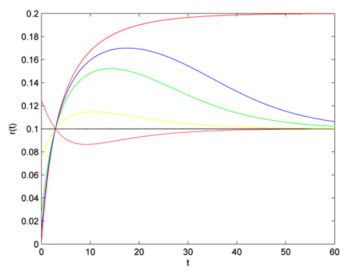 | Figure 4. Plots of hazard rate function |
According to Figure 3 and Figure 4, we can easily see that parameter  changes both the shape of probability density function and hazard rate function. Here, we believe that CFGMWEM can be used in interesting data groups that may pose two different types of risks.When parameter
  has a value between
  hazard rate function becomes bathtub shape. However, there are initial decreasing proportions of deaths, and at the beginning some components rapidly deteriorate. Thereafter a balance is formed and an almost constant hazar rate is observed. In the last part of the curve, components that complete their lifetimes are increasingly out of the system and the life span of the system is completed.When parameter
  has a value between
  hazard rate function becomes the opposite of bathtub shape. This curve is symmetric to value of parameter
  which is the hazard rate of exponential distribution. At the beginning, there are high risk, and initially some components are rapidly deteriorating. Thereafter a balance is formed and an almost constant hazar rate is observed. In the last chapter, components that complete their life span are decreasingly out of the system and the life span of the system is completed. This shape is called upside-down bathtub, inverse bathtub or unimodel.
2.1. Characteristics of Distribution
Moment generating function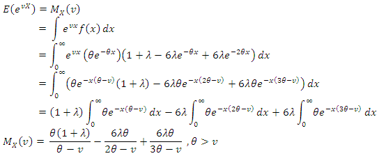 This is a linear combination of exponential distribution with
  and
and  mean. Through this, for
 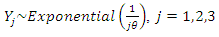 moment generating function can be written as
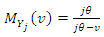
 | (3) |
k. th pure momentPure moments can be easily achieved with moment generating function. Expected value
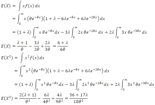 Variance
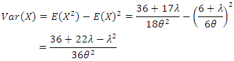
2.2. Moment Estimator
We find moment estimator with matching sample moments and pure moments of distribution. By this matching we can reach moment estimation under a condition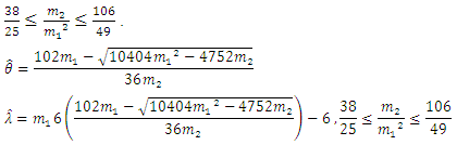
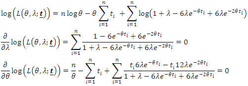
2.3. Maximum Likelihood Estimation
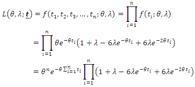 With using Log Likelihood, maximum likelihood estimation of parameters can be obtained with derivation of
  and
and 
2.4. L Moments Estimation
In  moments estimation we equalize
  samples to
  moments. Below we will first give
  samples and the calculations of these characteristics. After this we will give
  moments and their calculations. At last we will match them and find the estimations for parameters.Now we can express
  samples as follows.
  shows order statistics.
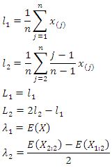 There are two equations with
  samples and
  moments matching.
 By using these two equations and adjusting them to CFGMWEM, the equations and matchings are observed as follows.
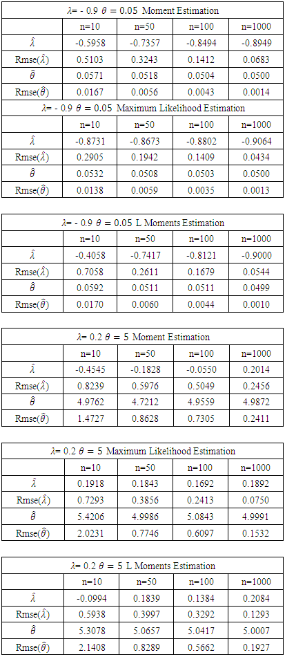
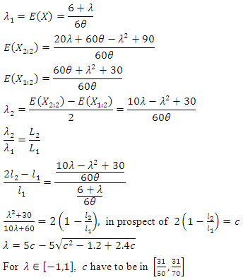 Now parameter estimation methods may be evaluated via examining Table 5. In Table 5 there are estimation results of three methods. Numerical technique is used for the results and repeating number is 100 for every observation.
  shows the observation number. Rmse is root mean squares of error.
 Table 5. Parameter estimation results
 |
| |
|
According to Table 5, maximum likelihood estimation is better than other two estimation methods. Because of this maximum likelihood estimation will be used in application part.
3. Results and Discussion
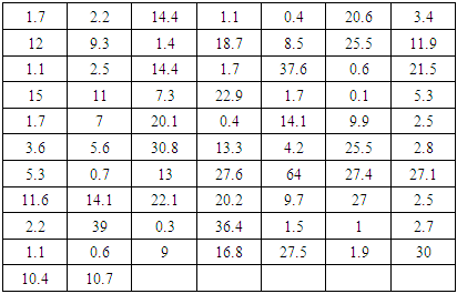
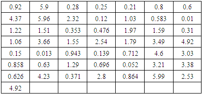
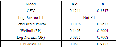
Now, using some different flow data, we first compare CFGMWEM with the most common hydrological statistical distributions. Subsequently, we offer CFGMWEM as a new distribution for flow data with different kinds of data groups. While comparing distributions, we will use Kolmogorov-Smirnov test statistics for looking the availability of our distribution to data sets. In Kolmogorov-Smirnov test statistics p value indicates the success rate of distribution in the explanation. [5], [8]Once we see that the two distributions are equal, we will have a new problem that which distribution is better for this data set. Because according to the hypothesis test, there may be many distributions that equal to nonparametric distribution. Akaike Information Criterion (AIC) can be used to compare these distributions. When AIC is used, the distribution with the minimum AIC value is selected as the best distribution. Since the AIC is a penalty value and the minimum value represents the maximum similarity to the non-parametric distribution of the data set, the minimum AIC value is the maximum similarity to the distribution. [1], [10] In this section, CFGMWEM will be compared with most known flow distributions using some different flow data. While comparing distributions, Kolmogorov-Smirnov test statistics will be used. When using Kolmogorov-Smirnov statistics, the least statistical value is considered to be the best modeling. p value of Kolmogorov-Smirnov statistics informs us about plausibility of the conformity.Data 1: The first data we used are the flood peak values (in m3/s) of the Wheaton River near Carcross in Yukon Territory, Canada. The data consist of 72 exceedances for the years 1958–1984, rounded to one decimal place. This data was analyzed in [2] and after this the same data was used in [4].Table 6. Wheaton River Flood Peaks (m3/s) data
 |
| |
|
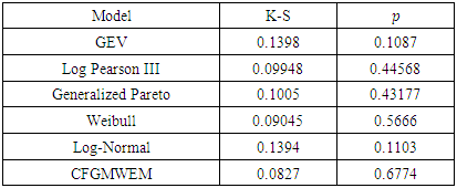
Table 7. Wheaton River Flood Peaks (m3/s) data test results
 |
| |
|
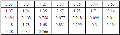
In terms of Table 7 CFGMWEM presents best model and clarifies data more than other distributions.Data 2: This data group is the values of Terme Creek's total flows in March from 1969 to 2000. The data group was received from Turkish State Water Affairs Directorate. In introduction section we told that there were two kinds of flow values that we looked for. These values are extremes and low flows. Therefore, we use the Terme Creek's total flows in March for extreme values analysis because it takes the highest values in March.Table 8. Terme Creek’s Total Flows
 in March data in March data
 |
| |
|
Table 9. Terme Creek’s Total Flows
 in March test results in March test results
 |
| |
|
In reference to Table 9, CFGMWEM presents second best model and clarifies data more than the other four distributions.Data 3: This data group is the values of Terme Creek's total flows in September from 1969 to 2000. In introduction section we told that there were two kinds of flow values that we looked for. These values are extremes and low flows. Therefore, we use the Terme Creek's total flows in September for low values analysis because it takes the lowest values in September.Table 10. Terme Creek’s Total Flows
 in September data in September data
 |
| |
|
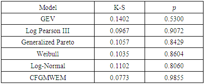
Table 11. Terme Creek’s Total Flows
 in September test results in September test results
 |
| |
|
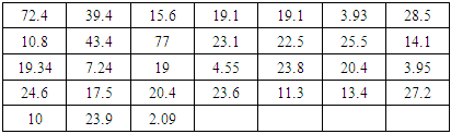
Given the results of Table 11 of the CFGMWEM, it is clear that CFGMWEM offers good models and can be used to estimate the data related to flows, as well as other distributions known as flow distributions.Data 4: This data group contains 56 measurements of total flows from Sefaatli Creek in April from 1953 to 2014. The data group was received from Turkish State Water Affairs Directorate. We use the Sefaatli Creek's mean flows in April for extremes analysis because it takes the highest values in April. Table 12. Sefaatli Creek’s Mean Flows
 in April data in April data
 |
| |
|
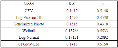
Table 13. Sefaatli Creek’s Mean Flows
 in April test results in April test results
 |
| |
|
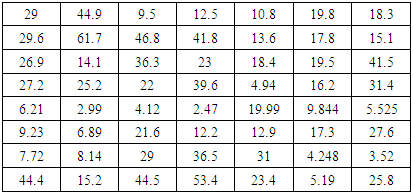
Data 5: This data group is the values of Sefaatli Creek's total flows in August from 1953 to 2005. The data group was received from Turkish State Water Affairs Directorate. In introduction section we told that there were two kinds of flow values that we looked for. These values are extremes and low flows. Therefore, we use the Sefaatli Creek's total flows in August for low values analysis because it takes the lowest values in August. Table 14. Sefaatli Creek’s Mean Flows
 in August data in August data
 |
| |
|
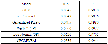
Table 15. Sefaatli Creek’s Mean Flows
 in August test results in August test results
 |
| |
|
In terms of Table 13 and Table 15, results point out the same conclusion with results of Terme Creek. Especially at low flows, CFGMWEM offers better modeling than other most common flow distributions.
4. Conclusions
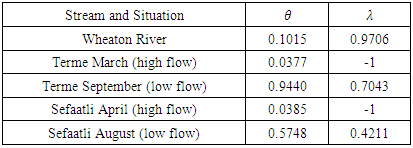
But how CFGMWEM conform with both extremes and low flows in the same time? Because these two kinds of data have completely different meaning. In part two we showed that the value of parameter  change the structure of CFGMWEM. So we want to show the values of this parameter in modeling. In Table 16 there are maximum likelihood estimation values for parameters in modeling data1 to data 5.
 Table 16. Values of Parameter Estimation in Models
 |
| |
|
We can easily see that when CFGMWEM gains conformity to extreme data,  parameter takes value between
  and when CFGMWEM gains conformity to low flow data,
  parameter takes value between
  According to test results for Data 1 to Data 5 we suggest that CFGMWEM can be used in every kinds of flows.We examine that CFGMWEM has best results in Data group 1, Data group 3 and Data group 5. For Data group 2 CFGMWEM has the second best results in modelling. And in modeling Data group 4 the new distribution has the third best results. According to Tables in application part we reach the conclusion that CFGMWEM can be identified as a stream distribution.
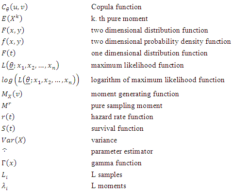
Notations
References
| [1] | Akaike, H. A New Look at the Statistical Model Identification. IEEE Transactions on Automatic Control., (1974). 19(6), 716-723. |
| [2] | Choulakian, V. and M.A. Stephens. Goodness-of-fit tests for the generalized Pareto distribution. Technometrics., (2001). 478-484. |
| [3] | Henderson, R. and Diettrich, J. Statistical analysis of river flow data in the Horizons Region: NIWA Client Report: CHC., (2007) 2006-154. |
| [4] | Merovci, F. and Puka L. Transmuted Pareto distribution. ProbStat Forum., (2014). 1-11. |
| [5] | Næss S. K. Application of the Kolmogorov-Smirnov test to CMB data: Is the universe really weakly random? Astronomy and Astrophysics (2012). A17, 1-4. |
| [6] | Nelsen, R.B. An Introduction to Copulas. New York: (2006). Springer. |
| [7] | Opere, A.O., Mkhandi, S. and Willems, P. At site flood frequency analysis for the Nile equatorial basins. Physics and Chemistry of the Earth., (2006). 31, 919-927. |
| [8] | Ross, S.M. Introduction to Probability and Statistics for Engineers and Scientists. Third Edition. Elsevier Academic Press: (2004). 504-514. |
| [9] | Sklar, A. Fonctions de repartition an dimensionset leurs marges. Publ. Inst. Statis. Univ. Paris,: (1959). 229-231. |
| [10] | Snipes, M. and Taylorn, C.D. Model selection and Akaike Information Criteria: An example from wine ratings and prices. Wine Economics and Policy, (2014). 3(1), 3-9. |
| [11] | Zaidman, M.D., Keller, V. and Young, A.R. Probability Distributions for “x-day” Daily Mean Flow Events. Bristol: Environment Agency., (2002). |

 Abstract
 Reference
 Full-Text PDF
 Full-text HTML