1. Introduction

The field, statistical design of experiments (DoE) was born in the 1920’s by the pioneering work of Fisher (2000) in the agriculture arena. A design for a two-level factor screening experiment constructed saturated design (SD) from orthogonal design if the number of factors, ‘p’ is equal to ‘n – 1’, where n is the number of runs. Some examples of saturated design are Plackett–Burman designs (Plackett and Burman 1946) [1] and p- efficient designs (Lin 1993) [2]. When p > n − 1, the design is called a supersaturated design (SSD). Supersaturated designs were introduced by Booth and Cox (1962) [3] and were not studied further until the important work of Lin (1993a) [4] and Wu (1993) [5]. Since then, much work has been done on this subject, recently by Bulutoglu and Cheng (2004) [6], Jones, Lin, and Nachtsheim (2008) [7], Bulutoglu (2007) [8] and Ryan and Bulutoglu (2007) [9]. A commonly used criterion defined by Booth and Cox (1962) [3] for choosing an SSD is the E(s²) criterion, including minimization of E(s²) or ave(s²) and minimization of maximum column correlation for evaluating and comparing designs. Nguyen (1996) [10] constructing two level supersaturated design from incomplete block design.

The concept of Orthogonal Array (OA) dates back to(Rao 1947) [11]. OAs has been used widely in manufacturing and high-technology industries for quality and productivity improvement experiments, as accounted by many industrial case studies and recent design textbooks (Montgomery 1997) [12]; (Wu and Hamada 2000) [13]. Applications of Nearly Orthogonal designs (NOAs) have been described by Wang and Wu (1992) [14]. From an estimation point of view, all of the main effects of an OA are estimable and orthogonal to each other, whereas all the main effects of an NOA are still estimable, but some are partially aliased with other (Honguan xu 2002) [15]. Since balance is an important and required property in practice, the balance considered in this article is OA (12, 3¹, 2⁹). The purpose of this article is to present a simple and effective construction of OAs and NOAs with mixed levels and small runs.

In this paper, we focus on finding combinatorial solution of the experiment. The experimental design considers an n× p matrix of factor settings, with a row corresponding to each of n design points and a column corresponding to each of p factors. This work has several steps, we clarify them as:

• We proposed a class of special super saturated design of the experiment which can be easily constructed via half fraction of the Hadamard matrices.

• We define mixed designs as designs with different factor types and different factor levels (e.g., factor 1 with 3 levels, factor 9 with 2 levels). Throughout this paper, we use the terms “qualitative” and “categorical” interchangeably, and may refer to discrete and continuous factors as “quantitative” or “numerical.”

• We checked the pairwise correlation (ρ) between any two factors (columns). An orthogonal design has ρ = 0. If a design has 0 < ρ ≤ 0.05, it is called a nearly orthogonal design.

• Finally, we analyze a design as efficient with optimality E (s²) and J₂ criterion if the number of design points is acceptable.

The purpose of this paper is to propose a framework for generating a design which is supersaturated design, nearly orthogonal and also balanced design with a minimum number of design points n. Section 2 articulates the Super Saturated design using Hadamard design in Thalassemic children. Section 3 shows that a solution for the problem which is an E (s²) - optimal SSD. Section 4 describes about an algorithm for constructing mixed-level OAs and nearly orthogonal designs (NOAs). Section 5 introduces the concept of J₂ -optimality and other optimality criteria. Section 6 contains concluding remarks.

2. Supersaturated Design Using Hadamard Design for Thalassemic Children

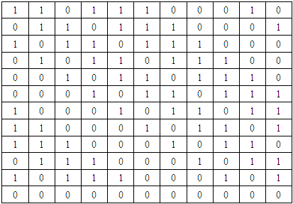
To have efficient analytical results a methodology for the design of an experiment was proposed in order to find as many as possible schemes containing maximum number of factors having different levels for the smallest number of experimental runs. This design study is based on an experiment which was conducted in order to obtain sufficient factors for accurate results. For the experiment, this study selected 250 Thalassemic children aged 8-18 years to analyze the impact of thalassemia disease and treatment pattern of thalassemic children.

Consider two-level factorial experiments with p factors and ‘n’ observations, n being even. Denote the two levels of a factor by + 1 and -1. Then the design is determined by, n X p matrix of elements and the ith column r_i gives the sequence of factor levels for factor ‘i’ in ‘n’ observations (1, 2, ..., n). We only consider the designs of the columns consisting of and Now in an ordinary factorial experiment, where we assume interactions being ignored, the efficient and simple estimation of main effects by calculating the orthogonality of all design columns (Plackett & Burman, 1946) [1] is ensured. So, the condition required is,

(1)

This condition cannot be satisfied for all i, j whenever p> n - 1; for otherwise the r_i , taken with a column of ones, would form a set of more than n orthogonal vectors in n dimensional space (Kathleen H.V. Booth and D.R. Cox, 1962) [3]. Therefore we require to have (1) satisfied as nearly as possible. First we require a minimum value for

(2)

The resulting design obtained is D-optimal design. D-optimal designs are straight optimizations based on a chosen optimality criterion and the model that will be fit. The optimality criterion used in generating D- optimal designs is one of maximizing |rr_i’|, the determinant of the information matrix rr’.

(Lin 1993) [2] proposed a class of special super saturated design which can be easily constructed via half fraction of the Hadamard matrices. These designs can examine K=N-2 factors with n=N/2 runs, where N is the order of the Hadmard matrix used. The (Plackett and Burmann1946) [1] designs, which can be viewed as a special class of Hadmard matrices, are used to illustrate the basic construction method of super saturated design in thalassemic children.

We are interested in studying the effect of some clinical variables on thalassemia children’s health using a subset of following 11 variables for super saturated design: Pale appearance (yes/no), Less appetite (yes/no), Frequent history of body temperature (yes/no), No weight & height gain (yes/no), Pneumonia (yes/no), Loose motion & vomiting (yes/no), Anxious Behaviour (yes/no), Less hemoglobin (yes/no), very weak/dull/less active (yes/no), frequently sick (yes/no), cough & cold (yes/no), Jaundice (yes/no), Previous history in family (yes/ no).

For this experiment a full factorial design with single replication would require testing children with the above mentioned factors. This appears to be an impossible task. The interest of the experimenter is to identify only important active factors. An efficient design was needed to investigate the important variables in the model. Even an orthogonal main effect plan would require test results obtained from 12 children (Hadamard matrix H₁₂). But for this test we would only require test results from 6 children (using SSD). The following design is a possible alternative for 6 runs obtained from Hadamard matrix H₁₂.

Table 1. The Plackett-Burman Design Run OA (12, 211), representing 11 two-level factors in 12 runs

Table 1 shows the original 12-run Plackett and Burmann design. If we take column 11 as the branching column, then the runs can be split into two groups, Group I with the sign +1 in column 11 and Group II with the sign -1 in column 11. Deleting column 11 from group I causes 1-10 columns to from a SSD to examine N-2=10 factors in N/2=6 runs. It can be shown that if group II is used, the resulting SSD is an equivalent one. In general a Plackett and Burman (1946) [1] design matrix can be split into two half-fraction according to a specific branching column whose sign is either +1 or -1. Specifically, take only the rows which have +1 in the branching column. Then N-2 columns other than the branching column will form a SSD for N-2 factors in N/2 runs. Judged by various design criterion, including E(s²) proposed by (Booth and Cox 1962) [3] then design have been shown to be superior to other existing SSD. Consequently, the E (s²) value for a SSD from half fraction Hadamard matrix is n² (n-3)/[(2n-3)(n-1)] which can be shown to be minimum within the class of design with same size.

Table 1.1. Binary codes of the Super saturated design

Wu (1993) [5] made use of such property and proposed a SSD that consists of all main-effects and two factors interaction columns from any given Hadamard matrix of order N. The resulting design has N runs and can accommodate up to N (N-1)/2 factors. When there are k (Ravindra Khattree, Calyampudi Radhakrishna Rao) [16].

By exploiting a relationship between SSDs and orthogonal designs (OA) presented in Section 2, we show that a solution for the problem is an E (s²) - optimal SSD with (n, m) = (6, 10) derived from a OA design with 12 treatments and 11 blocks.

3. E (s²) as a Measure of Goodness of Supersaturated Designs

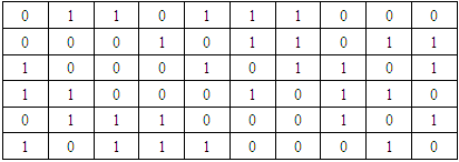
We present a method for constructing two-level supersaturated designs (SSDs) from orthogonal designs. A lower bound of E(s²) that also covers the case of odd run sizes is given. This bound is attained by SSDs constructed from orthogonal designs.

Let X be an n*p design matrix of a design with n runs and m two level factors each with 1/2n of +1 or high level value and 1/2n of -1 or low level values (p>n-1). Let S_ij be the element in the ith row and jth column of X’X. Booth and Cox (1962) proposed on a criterion for comparing design the minimization of ave(S²).

Where ave(s²) = Clearly the orthogonal design ave(S²)=0.

The rationale of the Booth-Cox criterion can be explained by using the singular value decomposition to decompose X as UA^1/2V’ where matrices U and V are orthogonal and A is diagonal. It can be shown that X’X and XX’ share the same set of non-zero eigenvalues (λ₁, ..., λ_r).

Where, r =rank(X’X)=rank(XX’). Moreover 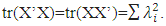Thus, minimizing which is equivalent to minimizing tr (X’X)²), is the same as making the λ_i ‘s equal as possible with = constant.

This in a sense is an approximation of the A-Optimality criterion, which requires the maximization of Because the sum of each column of X is 0, the sum of the elements of XX’ is 0 i.e. the sum of the off diagonal elements of XX’ equal to –np (np is the sum of the diagonal elements of XX’).

Thus, the sum of square of elements of XX’ and X’X will reach the minimum if XX’ is of the form (p-x) I_n+J_n where x=-p/n-1 (assuming p is divisible by n-1), I_n is the identity matrix and J_n is the n*n matrix of 1’s.

In this case ave (S²) = n (p²+ (n-1) x²-pn)/p (p-1) = n²(p-n+1)/(n-1)(p-1).

4. Construction of Nearly Orthogonal Design for Thalassemic Children

We assume that the research and development department of the health care wants to know whether there is a more economical design. Nearly Orthogonal design consider another study conducted to examine 12 factors affecting the children suffering with Thalassemia: Age of chelation therapy was started (less than 5 years, 1-5 years, above 5 years) Pale appearance(yes/no), Less appetite(yes/no), Frequent history of temperature(yes/no), No weight & height gain(yes/no), Pneumonia(yes/no), Loose motion & vomiting(yes/no), Irritation(yes/no), Less hemoglobin(yes/no), Very weak/dull/ less active(yes/no), frequently sick(yes/no), cough & cold(yes/no), Jaundice(yes/no), Previous history in family(yes/ no). To ensure that all the main effects are estimated clearly from one another, it is desirable to use an orthogonal array (OA). The smallest OA is found for one three-level factor and nine two-level factors. However, we want to reduce the cost of this experiment and plan to use a 12-run design. A good solution then is to use a 12-run nearly-orthogonal array (NOA).

Consider the matrix of Table: 2 below, of OA (12, 3¹, 2⁹) the first column has three levels and the other 9 columns have two levels each. For illustration w_k=1 is chosen for all k. Now we consider a design comprising the first five columns of OA (12, 3¹, 2⁹).

Table 2. The Design OA (12, 31, 29), representing first column has three-level and other factors have two level each

5. J₂ Optimality Criterion

The concept of J₂-optimality criteria for matrix d=[x_ik], weight w_k>0 is assigned for column k, which has s_k levels. For 1≤ i< j≤ N, let 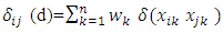, where if x=y and 0 otherwise.

The value measures the similarity between the ith and jth rows of d. In particular, if w_k=1 is chosen for all k, then is the number of coincidences between the ith and jth rows.

Define 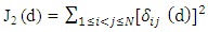A design is optimal if it minimizes J₂. By minimizing J₂(d), it is desired that the rows of d be as dissimilar as possible. The following lemma shows an important lower bound of J₂.

Lemma: For an matrix d whose kth column has s_k levels and weight w_k,

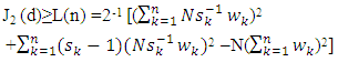(3)

and the equality holds if and only if d is an OA.

The statistical justification of J₂-optimality and other optimality criteria is given in the section. The coincidence matrix 12 rows is:

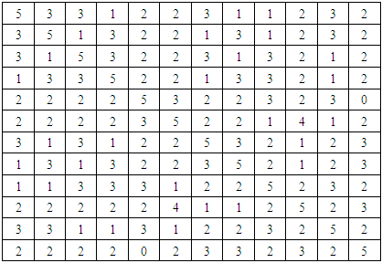It is easy to verify that J₂=330 and that the lower bound in (3) is also 330 for one factor have 3 level and four factor have 2 level column with w_k=1. Therefore, we consider the first five columns from OA (12, 3¹, 2⁹), because the J₂ value equals the lower bound.

Next, consider the whole array, comprising all 10 columns. Same calculation shows that J₂= 1284 and that the lower bound of (3) is 1260. Therefore, the whole array is not an OA because the J₂ value is greater than the lower bound.

6. Conclusions

The result of this paper enlightens us with an efficient construction method for Super Saturated and Nearly Orthogonal designs. An efficient design was needed to investigate or generate those variables and combinations which are important. In our study an orthogonal main effect plan would require clinical testing of 12 thalassemia children, but with super saturated design we can test only 6 children. The resultant arrays are optimal with respect to E(s²) and J₂ optimality criteria. Advantage of these constructions are:- eased usability, flexibility for constructing various mixed level designs to generate several OA’s main effect plans. The proposed construction method is important because it can efficiently construct more new Nearly Orthogonal and Supersaturated designs with good projective properties.

ACKNOWLEDGMENTS

We are grateful to an anonymous referee for their helpful and constructive comments.