-
Paper Information
- Paper Submission
-
Journal Information
- About This Journal
- Editorial Board
- Current Issue
- Archive
- Author Guidelines
- Contact Us
International Journal of Statistics and Applications
p-ISSN: 2168-5193 e-ISSN: 2168-5215
2019; 9(2): 45-52
doi:10.5923/j.statistics.20190902.01

A Study of the Ability of the Kernel Estimator of the Density Function for Triangular and Epanechnikov Kernel or Parabolic Kernel
 Abstract
 Reference
 Full-Text PDF
 Full-text HTML
Didier Alain Njamen Njomen, Ludovic Kakmeni Siewe
Department of Mathematics and Computer’s Science, Faculty of Science, University of Maroua, Maroua, Cameroon
Correspondence to: Didier Alain Njamen Njomen, Department of Mathematics and Computer’s Science, Faculty of Science, University of Maroua, Maroua, Cameroon.
| Email: |  |
Copyright © 2019 The Author(s). Published by Scientific & Academic Publishing.
This work is licensed under the Creative Commons Attribution International License (CC BY).
http://creativecommons.org/licenses/by/4.0/

In this paper, we are interested in the nonparametric estimation of probability density. From the « Rule of thumb » method, we were able to determine the smoothing parameter  of the Parsen-Rosenblatt kernel estimator for the density function. Our study is illustrated by numerical simulations to show the performance of the triangular core and Epanechnikov or parabolic density estimator studied.
Keywords: Density function, Smoothing parameter, Method of Rule of thumb
Cite this paper: Didier Alain Njamen Njomen, Ludovic Kakmeni Siewe, A Study of the Ability of the Kernel Estimator of the Density Function for Triangular and Epanechnikov Kernel or Parabolic Kernel, International Journal of Statistics and Applications, Vol. 9 No. 2, 2019, pp. 45-52. doi: 10.5923/j.statistics.20190902.01.
Article Outline
1. Introduction
- The theory of the estimator is one of the major concerns of statisticians. It is a fundamental element of statistics. It allows to generalize observed results. There are two approaches:× the parametric approach, which considers that the models are known, with unknown parameters. The law of the studied variable is supposed to belong to a family of laws which can be characterized by a known functional form (distribution function, density f, ...) which depends on one or several unknown parameters to estimate;× the non-parametric approach, which makes no assumptions about the law or its parameters.Knowledge about the model (non-parametric model) is not generally accurate, i.e., we do not have enough information on this model unlike the parametric model, which is often the case in practice. In this situation, it is natural to want to estimate one of the functions describing the model, either generally the distribution function or the density function (for the continuous case): this is the objective of the functional estimation.Since the works of Rosenblatt (1956) and Parzen (1962) on non-parametric estimators of density functions, the kernel method has been widely used in such works, as Prakasa Rao (1983), Devroye and Györfi (1985), Silverman (1986), Scott (1992), Bosq and Lecoutre (1987), Wand and Jones (1995), Benchoulak (2012), Roussas (2012) and the references cited in these publications. Based on the study of the local empirical process indexed by certain classes of functions, Deheuvels and Mason (2004) have established probability convergence speed for deviations of these estimators from their expectations.The central purpose of this article is to show the performance of the kernel density estimator for triangular and Epanechnikov or parabolic kernels.For us to attain this aim, the present article is divided into three (3) parts: firstly, as revision, we are going to introduce some different modes of convergences and give some Bernstein exponential inequalities which have permitted us to regulate the limit of deviations of the estimators compared to their hopes. This is why we will mention three (3) non-parametric methods of density estimation: the histogram method, the simple estimation method and the kernel method (Parzen-Rosenblatt estimator) on which will be our focus and which can be considered as an extension of the estimator by the histogram. We will also present the statistical properties of every estimation method. In the second part, using the Rule of thumb method (studied in Deheuvels (1977), and Sheather, Jones, and Marron (1996)), we will determine the
 smoothing parameter. Finally, using numerical simulations, we will explain the performance of the studied estimator.
2. Density Function Estimator
2.1. The Parzen-Rosenblatt Kernel Estimator
- For the fact
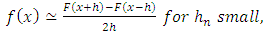 | (1) |
 , so:
, so: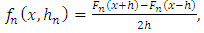 | (2) |
 is the empirical function of distribution. This estimator can also be written as:
 | (3) |
 .In this same article, Rosenblatt (1956) measured the quality of this estimator, by calculating its bias and its variance, given respectively by
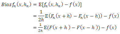 | (4) |
 | (5) |
 and
and  when
when  , we have:
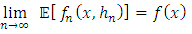 and
and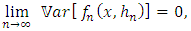 therefore,
  is a consistent estimator.By putting
 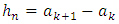 , we notice that the estimator of f on
  does not present the problem of the choice of origin
  as is the case of the histogram but it has the disadvantage of being discontinuous at points
  The generalization of this estimator had been introduced by Parzen since 1963 by performing
 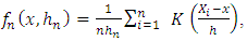 | (6) |
 , called window, is a strict sequence of positive real tending to zero when
  (called window) and K is a measurable function defined from
  , called kernel.
2.2. Properties of the Estimator
- The pillar of the first results of the convergence of this estimator is the theorem of Bochner (1955). The estimator kernel of the density depends on two (2) parameters: the window
 and the kernel K. The kernel K establishe he aspect of neighborhood of x and
  , controls the wideness of this neighborhood, so
  is the first parameter to have good asymptotic properties. Nevertheless, the kernel K must not be neglected. As the works of Parzen (1962) on the consistence of this estimator shows, this properties is obtained after having studied the asymptotic bias of the variance and the following decomposition:
 | (7) |
 ;(K.2)
 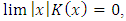 when
when  ;(K.3)
  , meaning that
 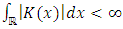 ;(K.4)
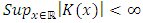
  ;(K.5) K is bounded, integrable and a compactly support.
2.2.1. Study of Bias
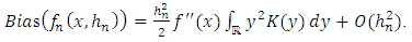
- The bias of
 is given by the following result:Proposition 1 (Parzen, 1962)Under the hypothesis (K.1), (K.2), (K.3) and (K.4) above, and if f is continuous, then:
 | (8) |
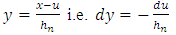
2.2.2. Study of the Variance of 
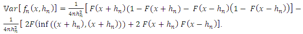
- The variance of
 is given by the following result:Proposition 2 (Parzen, 1962)Under the conditions K.1), (K.2), (K.3) and (K.4), and if f is continuous in all the points x of
  , then we have:
  | (9) |
3. Choice of Smoothing Parameter
- In this section, we study the choice of the smoothing parameter
 by the « Rule of thumb » method and give it’s result for the triangular kernel K and the Epanechnikov or parabolic kernel. In order to obtain these results, we determine at priori the mean and integral quadratic errors of
  .
.3.1. Method of the Mean Quadratic Error Criteria of 
- The mean square error (MSE) is a measure permitting the evaluation of the similarities of
 relative to the unknown density function f at a given point x of
  . Our aim being to minimize the following quantities:
 | (10) |
 | (11) |
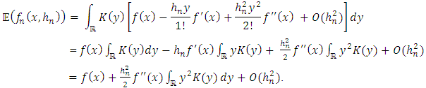
 : a) Calculating the Mean of
  The calculation of the means gives us:
 In putting:
  , we have:
  | (12) |
 , we obtain:
  | (13) |
 | (14) |
 | (15) |
 | (16) |
 | (17) |
 | (18) |
 The variance of
  is given by:
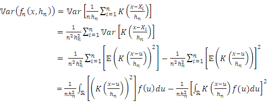 | (19) |
 , we have:
  Using an analogue working with the calculation of the mean above and using the Proposition 2, we obtain a new expression of the variance:
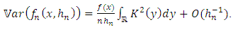 | (20) |
 | (21) |
 the expression of the Asymptotic Mean Squared Error (AMSE) given by:
 | (22) |
 is a solution to the equation:
  Thus, the smoothing parameter in the case of the estimator of the density function of the Parzen-Rosenblatt kernel is given by:
 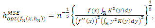 | (23) |
 c) Global ApproachWe will now focus on the global approach to select
  parameter. For this, we introduce the mean integrated square error (MISE) of
  . We obtain:
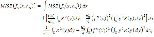 | (24) |
 Thus, the Asymptotic Mean Integrated Error (AMISE) is
 | (25) |
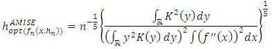 | (26) |

3.2. Method of Optimisation of 
3.2.1. Introduction
- There are several methods of optimizing
 in the literature. The most used are: The Plug-in method (Shealter, Jones, and Marron, 1996), the thumb method still called Rule of thumb (Deheuvels, 1977) and the method of cross validation (Rudemo, 1982; Bowmann, 1985 and Scott-Terrel, 1987). The method used in this article is that of Rule of thumb because it is best suited for calculating densities.
3.2.2. Rule of Thumb Method
- The optimal smoothing parameter with respect to the integrated root mean square contains the unknown term
 This method proposed by Deheuvels (1977) consists in supposing that
  is the Gauss density of mean 0 and variance
  , if we use the Gauss kernel, we obtain the window:
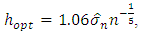 with
with  the emperical estimator of
  .If the true density is no’t Gauss, this estimation of the windows does not gives good results.
3.3. Fundamental Results
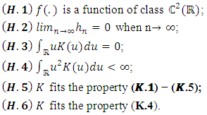
- To have our results, we will need the following hypotheses:
3.3.1. Triangular Kernel
- Let the triangular kernel be defined by:
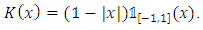 | (27) |
 and
and  , we have:
 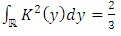 | (28) |
 | (29) |
 Similarly, we have:
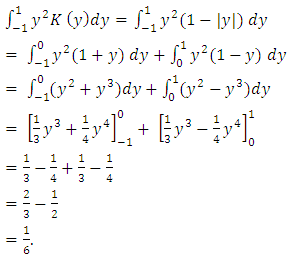 This fundamental result specifies the choice of the window
  of the triangular kernel by Rule of thumb method. Theorem: Under the hypotheses (H.𝟏) − (H.5) and if we choose f as the unknown normal distribution of mean 0 and variance
  , the value of
  is given by:
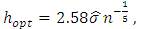 | (30) |
 and where
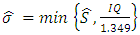
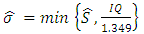
  is the estimator of the standard deviation and IQ is the estimator of the interquartile deviation.Proof The value of AMISE is given by:
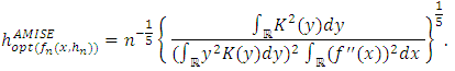 On the other hand, f being an unknown normal distribution of mean 0 and variance
  , we have:
 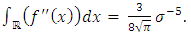 Thus,
Thus,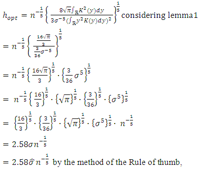 where
where 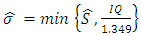 and where
  is the estimator of the standard deviation and IQ is the estimator of the interquartile deviation.
3.3.2. Epanechnikov Kernel or Parabolic Kernel
- Let the Epanechnikov kernel or parabolic kernel be defined by:
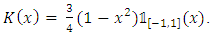 | (31) |
 | (32) |
 | (33) |
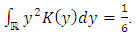
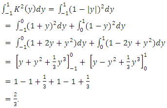
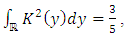
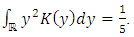
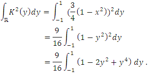 Finally, we have:
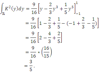 Similarly, we have:
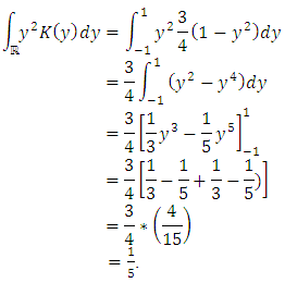 This fundamental result following precise the choice of the window
  and of the Epanechnikov kernel by the Rule of thumb method.TheoremUnder the hypothesis (𝑲.𝟏) − (𝑲.𝟓), and if we choose f like the normal unknown distribution of mean 0 and variance
  the value of
  is given by:
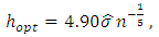 | (34) |
 and where
  is the estimator of the standard deviation and IQ is the estimator of the interquartile deviation.Proof The value of the AMISE is given:
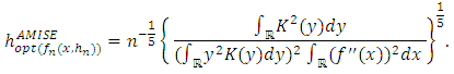 On the other hand, f being an unknown normal distribution of mean 0 and variance
  , we have:
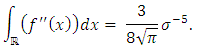 Thus,
Thus, 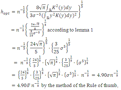 where
where 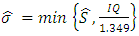 and where
  is the estimator of the standard deviation and IQ is the estimator of the interquartile deviation.
4. Simulation
- We present in this section a simulation study carried out using the R software, to try to illustrate the different theoretical aspects discussed in the previous section. This numerical illustration will allow us to see the result of the density estimation by the method of the Role of thumb of the smoothing parameter.
4.1. Introduction
- We consider a sample
 , series of random independent and identical distributed variables (i.i.d) of probability density f which obey the law
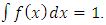
 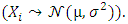 To estimate f in a given interval, we suppose that F represents the function of distribution and f their density function in the form:
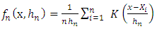 where K is the chosen kernel and
  is the window parameter.If K is a triangular kernel, then the value of optimal
  noted
noted  is given according to section 3.3.1 by:
 On the other hand, if k is a parabolic or Epanechnikov kernel, then the value of optimal
  noted
noted  is given according to section 3.3.2. by:
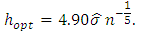 We will generate for every of the applications which we propose the samples of height
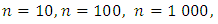
 respectively.
4.2. Simulation Algorithm
- In other to simulate the sample defined above and to evaluate the performances in a given interval, we go through the following steps:1. Generate the sample
 according to the normal law;2. Give the number of observation n of the simulation;3. Give the interval of the simulated space;4. Choose the kernel
  ;5. Choose the smoothing window
  ;6. Estimate
  with their estimator;7. Draw the graph of the estimated densities.
4.3. Results of Simulation
- The following simulation curves obtained in this section are conceived in the software R. the construction codes are given in the annex.
4.3.1. Triangular Kernel
 | For n = 10, we have the following graph: |
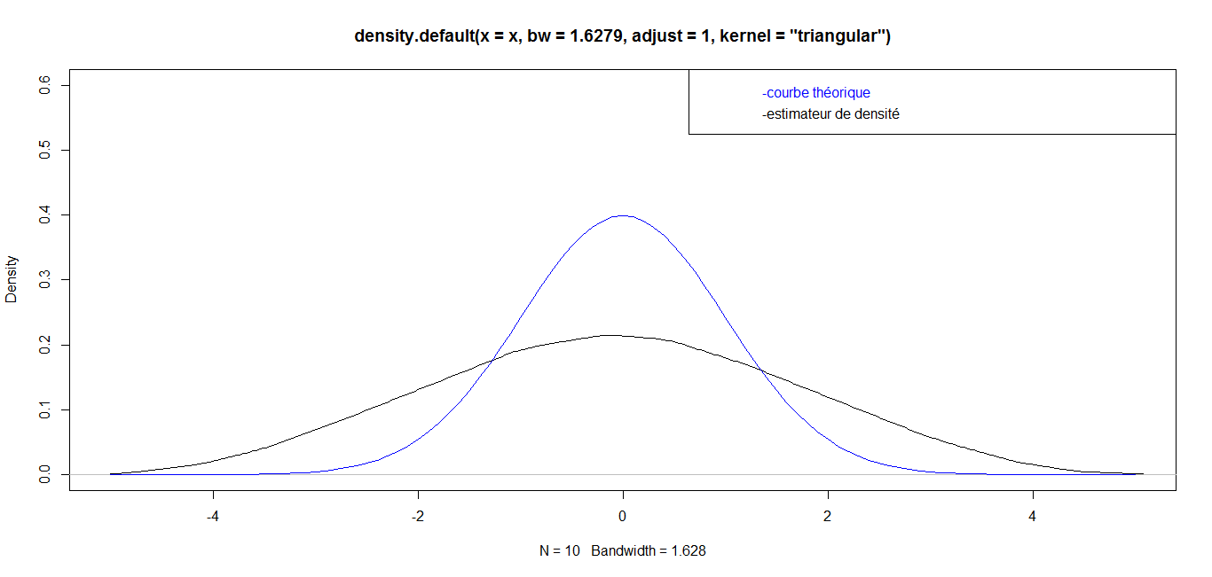
 | For n = 100, we have the following graph: |
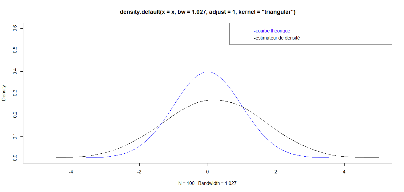
 | For n = 1 000, we have the following graph: |
 | For n = 10 000, we have the following graph: |
 | For n = 100 000, we have the following graph: |
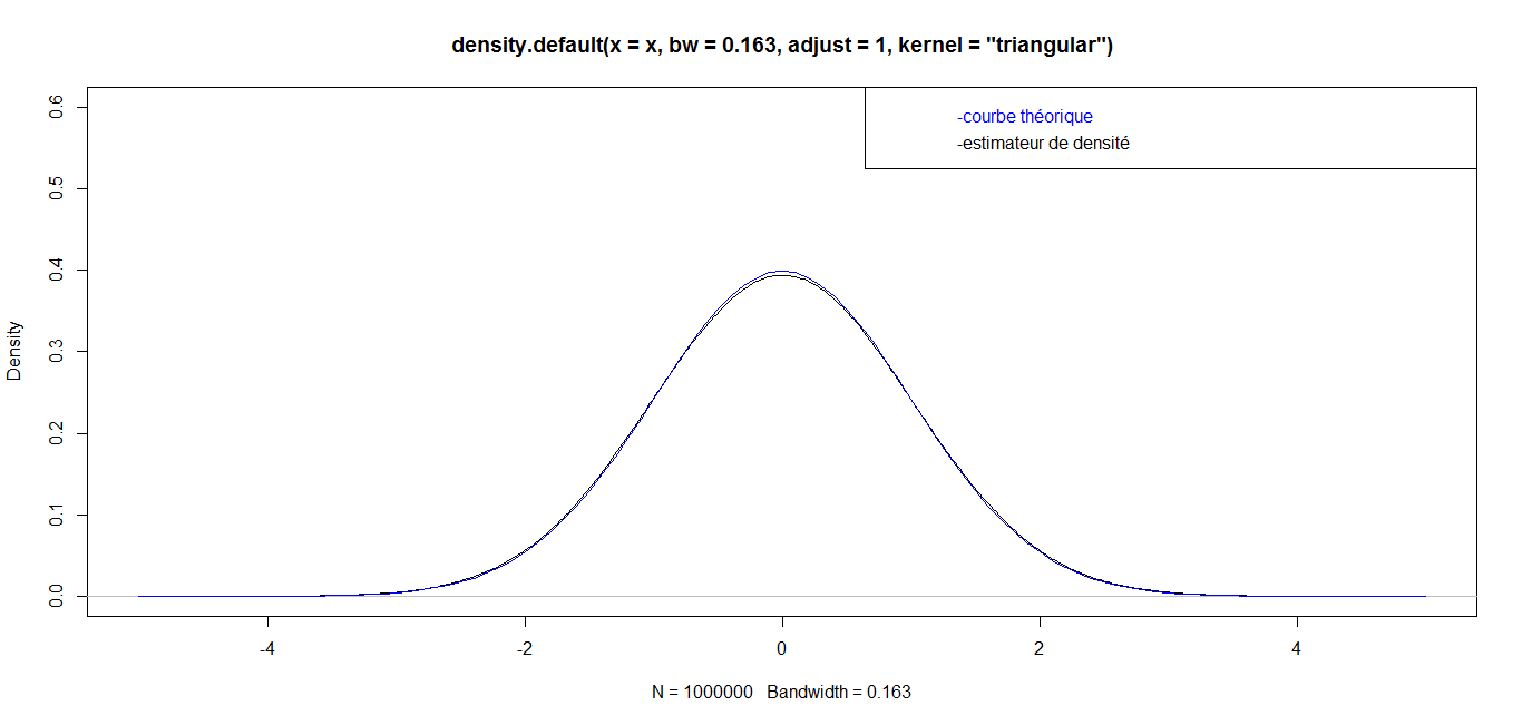 | For n = 1 000 000, we have the following graph: |
 while for great values
  they are almost identical. Finally, for a very big value (n=1 000 000), the curves are identical, which confirms the robustness of our density estimator in the case of triangular kernel.
 4.3.2. Epanechnikov Kernel or Parabolic Kernel
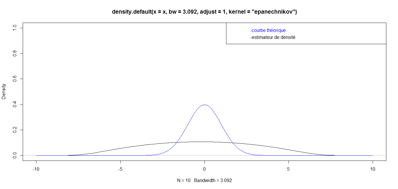 | For n = 10, we have the following graph: |
 | For n = 100, we have the following graph: |
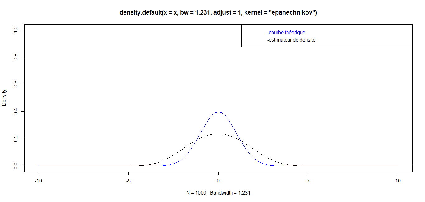 | For n = 1 000, we have the following graph: |
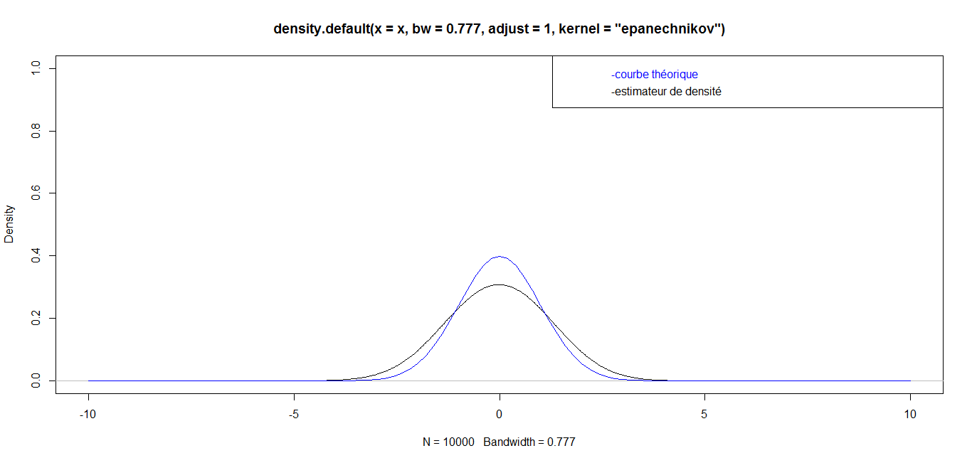 | For n = 10 000, we have the following graph: |
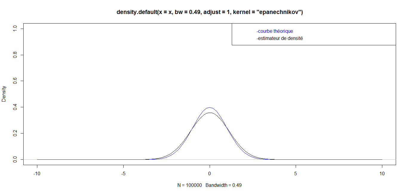 | For n = 100 000, we have the following graph: |
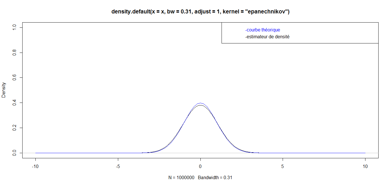 | For n = 1 000 000, we have the following graph: |
5. Conclusions
- In this paper, by studying the nonparametric estimate of the probability density of the triangular core and the Epanechnikov kernel by the "Rule of thumb" method, we have succeeded in determining the smoothing parameter
 of the kernel estimator of Parsen-Rosenblatt. We notice that when we increase the number of observations N, the error decreases and the information of the estimator is almost the same as the theoretical information. The results obtained from the software R perfectly illustrate this reduction of the error. By comparing them, we clearly see that the shape of the Parzen-Rosenblatt estimator approaches the shape of the theoretical probability density when the number of observations N increases and the window h decreases. In general, the performance characteristics obtained in the different observations of this sample with the Parzen-Rosenblatt estimator are very close to the theoretical ones. The higher N is, the better the estimate of densities.We plan to study the kernel estimator of Nadaraya-Watson using the regression function and evaluate the quality of the estimation, to treat the asymptotic properties of these estimators, namely the convergence in quadratic average. This will allow us to study the convergence almost complete punctual as well as uniform.The study of this kernel estimator of the Nadaraya-Watson density function will be studied in the context of competiting risks such as defined by Njamen and Ngatchou (2014) in order to compare the robustness of the two methods.
ACKNOWLEDGEMENTS
- The authors gratefully acknowledge the reviewers who reviewed this article.