Raymond Nero1, Oduro F. T.1, Abonongo John2
1College of Science, Department of Mathematics, Kwame Nkrumah University of Science and Technology, Kumasi, Ghana
2Faculty of Mathematic Sciences, Department of Statistics, University for Development Studies, Navrongo Campus, Ghana
Correspondence to: Raymond Nero, College of Science, Department of Mathematics, Kwame Nkrumah University of Science and Technology, Kumasi, Ghana.
| Email: |  |
Copyright © 2019 The Author(s). Published by Scientific & Academic Publishing.
This work is licensed under the Creative Commons Attribution International License (CC BY).
http://creativecommons.org/licenses/by/4.0/

Abstract
Survival analysis is employed in estimating the survival proportions of infants born in the Nandom district, Ghana and the infant mortality count data fitted to four standard loss distributions. The four loss distributions were Poisson, Binomial, Negative Binomial and Geometric distributions. The results showed that, the first twenty-four (24) hours and month after delivery are the most critical periods in the life of an infant child in the Nandom District. Also, about 98 percent survived up to the neonatal stage and only 97 percent made it to the post neonatal stage. The conditional proportion of infants dying within the early neonatal stage recorded the highest proportion of about 2.17 percent. The Negative Binomial Distribution was the best model to fit the infant mortality data with log-likelihood and A.I.C values as -31.7365 and 65.4730 respectively with an expectation of about 51 deaths per year. This implies that, the district is still facing a bigger challenge in terms of infant mortality and should therefore work towards achieving the goal as stipulated in the SDGs.
Keywords:
Survival analysis, Infant mortality, Maximum Likelihood estimate, Life table
Cite this paper: Raymond Nero, Oduro F. T., Abonongo John, Survival Modeling of Infant Mortality. Evidence from Nandom District, International Journal of Statistics and Applications, Vol. 9 No. 1, 2019, pp. 29-35. doi: 10.5923/j.statistics.20190901.04.
1. Introduction
In recent time past, Infant Mortality ratios were crucial indicators for the attainment of the Millennium Development Goals MDG 4 and 5 for all countries in fulfillment of the 2 out of 3 health goals from the 8 targeted on development and poverty eradication. The fourth MDG goal targeted at reducing the mortality rate of children under-five years by two thirds between 1990 and 2015 and as well make reproductive health accessible to all.However, from the trends of events unfolding, achieving these health Millennium Development Goals was a great challenge as many countries seems not to be on track to meeting their target by 2015[12], thus the business still remains unfinished. With the business being unfinished, a global leadership on poverty eradication, inequality and climate change became eminent and hence the formulation of the sustainable development goals.In an attempt to put a permanent end to poverty everywhere, world leaders convened a meeting at the United Nations in New York in 25th September 2015 in order to adopt another 15 years’ program that will put the world on a sustainable path. This post-2015 agenda comprises 17 new Sustainable Development Goals (SDGs) formulated to finish the job of the MDGs. That is to guide both policy and funding for the next 15 years. The MDGs 4 is now incorporated into MDG5 as SDG 3 which seeks to ”ensure healthy lives and promote well-being for all at all ages”. Target 1 of the SDG3 is to ensure a reduction of global MMR to less than 70 deaths per every 100000 live births by twenty countries focusing at reducing neonatal mortality to at least as low as 12 per 1000 live births and under 5 mortality to at least as low as 25 per 1000 live births.Infant Mortality is however, defined as the death count of children under age one. It is usually estimated using the Infant Mortality Rate (IMR). It describes the number of deaths of children below one year of age out of every 1000 live births. With an estimated nine-million children still dying each year before they reach their 5th birthday [14], majority of infant deaths occur in the first 28 days of life, with an estimated 3.027 million deaths representing 40.3 percent [9]. ”Progress towards the reduction of neonatal deaths has been slow, with little evidence of progress” [11].In the year 2015, 4.5 million (75 percent) of all under-five deaths happened within the first year of life. The risk of a child dying before completing its first birthday was highest in African countries (55 per 1000 live births), over five times higher than that in European countries which recorded 10 out of 1000 live births [15]. In Ghana, the IMR is 38.52 deaths per 1000 live births (CIA fact book), this still represents a great challenge as the SDG goals place more emphasis on survival (that is zero child deaths).Survival being the compliment of death, calculating the proportion of infants who lived past a certain time and the rate they fade out are taken into account in this paper. As Ghana meets the rest of the world to embrace the set of sustainable development goals, and to zero down mortality, the effect of population ageing coupled with high fertility (4.2 children per woman)? May seem to pose a hindrance towards reducing infant deaths to the barest minimum, hence the need for survival analysis to see what proportions of infant that will survive pasta certain age? And what proportion will die before reaching the same age? A loss distribution will be fitted to the infant mortality count data. This will help inform intervention strategies in the Nandom District of the Upper West Region of Ghana. Not only does the rapid ageing of population make the subject Mortality and its converse of Survival analysis worth studying, but also, infant and maternal health is important in its own right; as every person, mother or child alike deserves the right to live; counting on the fact that most of these deaths that brazen most countries out from hitting their MDG targets are preventable.Analysis of infant mortalities becomes a central problem, especially when coordinated efforts of districts and regions to meet the set of sustainable development targets of reducing infant deaths in the country was defeated. [6] Using the Logistic Regression, modeled the Risk Factors of Neonatal Mortality in Ghana using data from the 2008 Ghana Demographic Health Survey by the Ghana Statistical Service. In this study, three models were developed one each for mother level factors, child level factors and environmental factors. The results showed that, for the mother level factors, age and wealth index were the risk factors identified and associated with neonatal mortality in Ghana. Child size, sex and the number of children born of a single mother at birth at the child level factors did not show significant result of causing neonatal deaths while for at the environmental factor level, the location by region was found to be a factor contributing to neonatal mortality. From the findings drawn from the environmental factor level, it was established that poverty contributed towards neonatal deaths.[10] applied time series models to data on under-five mortality rates in Ghana from 1961 to 2012 year period to model the decrease in under-five mortality. The Box-Jarkins ARIMA model, Bayesian Dynamic Linear model and the Random Walk with Drift model were constructed for data value from 1961 to the year 2000 and an in- sampling forecasting is made for the subsequent years up to 2012. The random walk with drift was found to have fit the data well and was used for an out-of-sampling forecasting for the year 2013 through to 2016. The result showed a forecasted under-five mortality rate of 64 deaths per 1000 live births for the year 2015 which meant that Ghana would not be able to achieve the millennium development target of 42.7 death per 1000 live births by the end of the 2015.Guided by the singular objective to obtain a model for forecasting the death counts of children in families of Bangladesh, [2] employed four discrete loss distributions (Negative Binomial Regression (NBR), Zero Inflated Negative Binomial Regression (ZINBR), Hurdle Regression (HR), and Poisson regression) to count the response, death counts of children and to identify the risk factors. It was established that the death count of children in a family were positive count dependent variable. The average death count of children was found to be 28 per 100 women with a variance of 44 per 100 women. Thus Poisson regression model was not a good choice to predict the mean response from the Bangladesh DHS data due to the presence of over-dispersion. In order to address over dispersion, the Zero-Inflated Negative Binomial Regression (ZINBR) was the best model that fitted the data well. The Negative Binomial Regression (NBR), and Hurdle Regression (HR) model were also good fits. It was established that respondent’s socio-economic factors as well as demographic factors and environmental factors were identified as significant predictors for the number of children’s death in a family based on Zero-Inflated Negative Binomial Regression (ZINBR). It was recommended that ‘knowing the risk factors of the number of children’s deaths are of importance to public health issues and should be carried out meticulously for the much needed intervention”.In attempt to forecast the Rate at which Infant Mortality is declining in South Asia, [4] asked the following research question about South Asian countries; (1). What is the progress in reducing the IMR to meet the MDG target? Despite the time series data showed declining trends, in essence do such trends account for average annual progress? (2). can stochastic or deterministic trend explain the IMR decline. If so, what alternative time series model can be used to forecast the declining rate of Infant Mortality? and if a serviceable representative model for the entire region be concluded on? (3) if there were models that could adequately represent the entire region, how will the problem of forecast accuracy using the model and the propagation of forecast error be accounted for? In this approach, a Random Walk Approximation was used. The Logarithm of decline rate of infant mortality as a time series and fit alternative parametric time series models were considered. Partial Autocorrelation Function (PACF) and Auto Correlation Function (ACF) were used to assess stationary status of all the series which showed persistent patterns of sample ACF for all the countries. It was purported that for a liner relation, the autocorrelations did not approach zero. Hence ARIMA modeling of the first differences of these series was explored; ARIMA (p,1,q) models were considered. Based on residual checks, ARIMA(1,1,1), ARIMA(2,1,0), ARIMA(1,1,2) etc., were not acceptable. A random walk model and/or a ARIMA (1,1,0) was seen to have fitted well. In Comparison, ARIMA (1,1,0) chosen as adding more parameters favor the process. It was observed that linear extrapolation of IMR using the past rate may under or over estimate the shortfall in achieving the MDG child mortality target (see goal 4). It was cited that linear extrapolation of IMR for Bhutan has average annual reduction rate of 36 deaths per 1000 live births between 1990 and 2010, hence suggested that it would over exceed the MDG 2015 target. However, the ARIMA model indicated that there can be a shortfall to the extent of 11 percent with approximately 1 percent of error, so was the case, for the entire region of South Asia. The shortfall was under estimated by about 28 percent. It was believed that possibility of finding a time series model which was representative of the entire region of South Asia for the purpose of forecasting IMR decline which country level comparisons and stagnation monitoring of progress are made possible was demonstrated.Similarly, [5] modeled the contribution of birth intervals to infant and child mortality within the context of community framework. The study revealed that short birth interval (less than 72 weeks) affects infant and child mortality greatly when compared with long birth interval ( greater than 96 weeks), it means that contribution of short birth interval was severe on infant mortality as against child mortality. It was agreed that the maturity level of mothers had greater impact on infant and child mortality in general. Education was also unfolded to contribute significantly to infant and child mortality.The purpose of this paper is to model the survival of infant and as well fit a standard loss distribution to infant mortalities data of the study area. The loss distribution is commonly used to examine risk and the frequency or severity of the risk. This loss distribution approach is to help our health institutions develop mathematical models to enable them solve their mortality problems in Nandom Distict and Ghana at large.
2. Materials and Method of Analysis
2.1. Source of Data
Secondary data was collected from Ghana Health Service, Nandom District Health Directorate precisely for the period of 2008 to 2015. The information was collected in two folds, information on newborns was gathered for the period and it is assumed that the children were monitored from day one to the end of the first year of live and secondly, infant count mortality data was also sorted.
2.2. Methods of Data Analysis
2.2.1. Survival Times
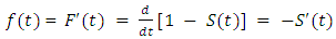
Survival times measure the time to a given event such as time to failure of a machine, divorce, student drop out, arrest time, development of a disease, relapse, or response. In this paper, the survival times measure the mortalities of Infants of Nandom District, in the Upper West Region of Ghana. The distribution of survival times is usually characterized by three functions: Survivorship function, S(t), the probability function, f(t) and the hazard function, h(t) [7].
2.2.2. The Survival Function, S(t)
Let the continuous random variable T measure the survival time of an infant child, where T is a non - negative real integer. It is considered that subjects are a random sample from a larger population of infant and that the actual survival times of individuals in a group is the value of the variable T. The Survival Function conventionally denoted S(t), is defined as the complement of the lifetime distribution function, F(t). It is the probability that an infant who is born survive longer than t. That is; | (1) |
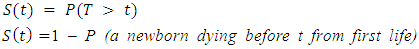 | (2) |
 | (3) |
 is a non increasing function of time with properties
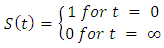 | (4) |
2.2.3. Probability Density Function (PDF)
This is defined as the limit of probability that an infant dies within the short interval  per unit time. It is represented mathematically as;
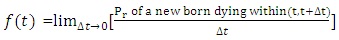 | (5) |
 | (6) |
In terms of survival functions,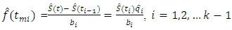 | (7) |
 is the cumulative proportion by time,
  within the
  interval. It is referredto as the cumulative survival rate. It implies that those infants surviving to the
  interval survived to the start of and through the
  interval. Thus,
 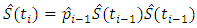 is the proportion surviving by time,
  with the
  interval.
 Typically defines the conditional probability of an infant dying in the
  interval given the number exposed to the risk at time,
  It is estimated using;
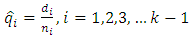 | (8) |
The conditional survival proportion  is given as
 is the width of the
  interval
 the midpoint of each interval
 = number dying in the
  interval
 = number exposed to risk in the
  interval
2.2.4. Hazard Function
The hazard function  is defined as the event rate at time
  conditional on survival until time
  or later. Suppose that a subject has survived for a time
  and we desire the probability of survival for an additional time,
  . Mathematically, it can be expressed as
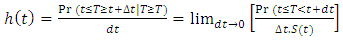 | (9) |
 | (10) |
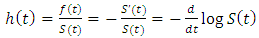
The hazard functions or hazard ratio synonymously called failure rate or force of mortality in actuarial literature, is the probability density function of the distribution. It is defined as;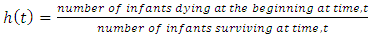 | (11) |
The hazard rate is the rate of death for lives aged  For a life aged
  , the force of mortality
  years later is the force of mortality for a
  years old. Actuaries often use the average hazard rate of the interval, which is the number of patients dying in the interval per unit time divided by the average number of survivors at the midpoint of the interval.
 | (12) |
Since the hazard is estimated at the midpoint, conventionally, the estimate is defined as;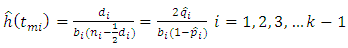 | (13) |
Equation 12 gives a higher estimate of hazard rate than the equation 13 and thus a more conservative estimate [10]. Assuming that the hazard rate is constant within an interval but varies among interval, [13] is of the view that the hazard function can be estimated using | (14) |
Which satisfies;  and
and  .
.
2.2.5. Survivorship Function Estimation
There are a number of ways of estimating survival functions, some of which includes the Kaplan-Meier and the Life Table Method. | (15) |
This is called the Kaplan-Meier Product Limit Estimator of survivorship.
2.3. Discrete Distributions under Consideration for Infant Count Mortality Data
2.3.1. The Binomial Distribution
A random variable X has the binomial distribution with parameters n and p if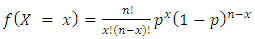 | (16) |
[10] are of the view that the probability distribution is called the binomial distribution because for 
 the values of the probabilities are the successive terms of the binomial expansion
  The CDF of the distribution is given as:
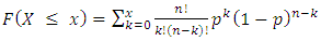 | (17) |
The likelihood function  is given by:
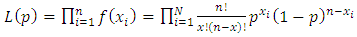 | (18) |
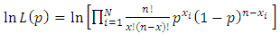 | (19) |
Setting the derivative of equation (19) to zero, the maximum likelihood estimate becomes: | (20) |
If  has the binomial distribution with parameters
  and
and  then
then 
2.3.2. The Poisson Distribution
A random variable X has the Poisson distribution with parameter  ifits probability mass function is given by:
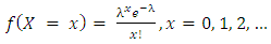 | (21) |
The Poisson distribution is used as a model for describing the number of times some random event occurs in an interval of time or space.λ is the average number of times the event occurs in the given time interval.The CDF of the Poisson distribution is given as;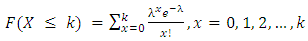 | (22) |
The likelihood function becomes: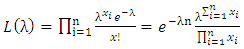 | (23) |
Setting the derivative of the log-likelihood of equation (23) with respect to  to zero, we obtain the maximum likelihood estimate as:
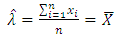 | (24) |
If  has the Poisson distribution with parameter
  , then
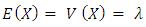 | (25) |
2.3.3. Geometric Distribution
In a series of independent Bernoulli trials, with constant probability p of success, let the random variable X denote the number of trials until the first success. Then X has the geometric distribution with parameter  and
and | (26) |
The CDF of the geometric distribution is given as: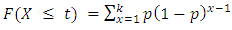 | (27) |
The likelihood function is given by: | (28) |
Setting the derivative of the log-likelihood of equation (28) with respect to  tozero, the maximum likelihood estimate becomes:
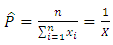 | (29) |
If X has the geometric distribution with parameter p, then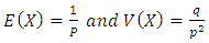 | (30) |
2.3.4. The Negative Binomial Distribution
In a series of independent Bernoulli trials, with a constant probability p of success, let the random variable X denotes the number of trials until k success occurs. Then, X has the negative binomial distribution with parameters  and k = 1,2,3,...Thus, the pdf becomes:
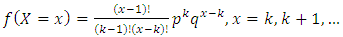 | (31) |
When  in equation (23), the distribution becomes geometric with parameter p. The negative binomial distribution is therefore a generalization of the geometric distribution, [10].The CDF of the negative binomialis given as:
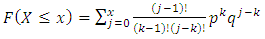 | (32) |
The likelihood function becomes: | (33) |
Setting the derivative of the log-likelihood of equation (33) with respect to p to zero, the maximum likelihood estimate becomes: If X has the negative binomial distribution with parameters p and k, then
2.4. Determination of the Appropriate Model
In identifying a distribution to describe infant mortality data, it is of prime importance that the data set can be best described by the properties of the theoretical distribution. In this paper, the method of maximum likelihood estimates was used to find a mathematical model(s) that describes infants’ mortality data. Goodness-of-fit test is done by the use of the A.I.C to further affirm the decision by MLE.
2.4.1. The Maximum Likelihood Estimator
[1] indicates that the method of maximum likelihood estimates is widely used because of its enormous properties and some of which includes: consistency, efficiency, asymptotic normality and invariance.Let  be the
  infantdeath,
 the number of infant deaths
 the likelihood function
 is the parameter
 the probability distribution function of a specific distribution.The likelihood function is given by:
 | (34) |
Differentiating equation (26) above is the result of the MLE; | (35) |
Equate equation (35) to zero to solve for the value of the parameter: To drive the maximum likelihood estimators is to formulate the statistical models in the form of a likelihood function as a probability of getting the data at hand [1].The likelihood estimates were derived for each of the seven statistical distributions according to the data set with the help of the R statistical package. The log-likelihood values obtained from the method of maximum likelihood estimates are compared to choose one model amongst the seven probability distributions considered in this research. The greater the likelihood the better the model.
2.4.2. Accessing the Adequacy of the Model
It is not appropriate to base on only the values of the log-likelihoods obtained to determine the best distribution hence a further check is required. An assessment ought to be done to check on how good the model will fit the infant mortality data. This research will therefore consider the goodness of fit test by the use of Akaike’s Information Criterion (A.I.C).The Akaike’s Information Criteria (A.I.C)The A.I.C criterion is defined by [3] as: | (36) |
Thus, it is used to test for the goodness of fit after having obtained the values of the log-likelihood in this research.
3. Results and Discussions
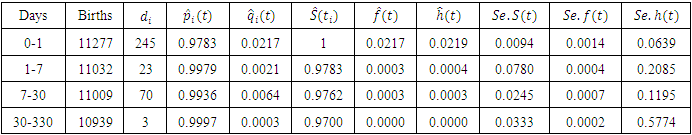
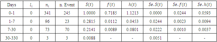
Survival analysis basically monitors a cohort from the beginning of a study to the end of the paper and thus note when each member of the group will fail. In this paper, the cohort constitutes newborns for a period of one year and they are followed on daily bases to the end. From the data obtained within the period under consideration, 11277 children were born and out of this 341 deaths occurred. In estimating the infant survivorship and failure proportions in the Nandom district, a script is built for the columns of the life table. The data is collected on daily bases and it is a right censored data. The infant count data is used to fit the distributions whiles the data on the births and deaths is used for the survivorship. Table 1 below shows an eleven column life table across different survival time intervals from birth through to 11 months (330 days) for infants in the Nandom district of the Upper West Region of Ghana. The fourth column of the life table estimates the conditional probability of an infant child surviving within the time interval. These estimates reveals that, while approximately 99.97 percent, 99.36 percent, 99.79 percent of infants born in the Nandom district survive within the post-neonatal period (30 to 330 days), neonatal period (7 to 30 days) and early neonatal period (1 to 7 days) respectively, about 98 percent survive within the first day of life. The conditional proportion of infants dying within the early neonatal period, neonatal period and post-neonatal period were approximately 2.17 percent, 0.21 percent, 0.64 percent and 0.03 percent respectively as shown in the 5th column.Table 1. Life Table for the Survival Proportions of Infants in the Nandom District
 |
| |
|
Column six (6) defines the cumulative survival proportion of infants in the district. Those infants that survived within the interval 0 to 1 survived at conception through to delivery with a probability of 1 and those that survived within the interval 1 to 7 days survived through delivery to the start of the first day of life with survival probability of 0.9783. Similarly, those that survive in the interval 7 to 30 and 30 to 330 days survived to the beginning of the interval with survival probabilities 0.9762 and 0.9700 respectively. The probability density function in the 7th column provides estimates of the unconditional probability of dying in the time interval per unit width. It is estimated at the mid-point of the time interval, hence the probability of an infant dying at mid-interval in the time interval 0 to 1, 1 to7, 7 to 30, 30 to 330 are respectively 0.0217, 0.0003, 0.0003 and 0.0000.The results further showed that approximately 99.78 percent of infant born in the Nandom district survive within their first day of life. Of the proportion of infant that survive their first day of life, only 99.36 percent make it to the end of the neonatal period while a 99.97 percent make it through to the end of post neonatal stage. Infants born on the first day have about 2.17 percent chance of dying between delivery and the first day of life. Given that a child survive the first day of life, it has approximately 0.21 percent chance of dying between the first day of life to the end of the first week and 0.64 percent chance from the first week to end of the first month and then 0.03 percent chance of dying within the first and eleventh month after delivery. This makes the first; twenty-four (24) hours, week and month after delivery the most critical period in the life of an infant child. It is assumed that all 341 infants were followed till the end of infancy and that the failure times recorded in the time interval are accurate.Table 2 shows the life table of infant mortality in the Nandom district. It could be seen that, the hazard occurred in the first; day, week and month with the first 24 hours being the most critical period in the infant’s life.Table 2. Life Table for 341 Infant Failures in the Nandom District
 |
| |
|
3.1. Fitting Infant Mortality Count Data
3.1.1. Maximum Likelihood Estimates of Infant Mortality Count Data
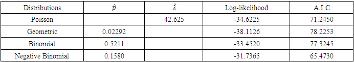
Table 3 shows the parameter estimates of infant mortality count data. The results show that among the four distributions, the Negative Binomial distribution had the highest log-likelihood value of -31.7365 and with the least AIC value of 65.4730 and therefore was selected as the best distribution to fit the infant mortality count data. Table 3. Results of Parameter estimates of Infant Mortality Count Data
 |
| |
|
4. Conclusions
The life table method; a non-parametric method which provides estimates of the Kaplan-Mier product limit estimation was used to estimate the survival proportions of infants. The method of maximum likelihood estimate and Akaike’s Information Criterion were used to affirm the best model to fit the mortality count data. From the survival analysis performed on infant time till death data, the results showed that, while about 98 percent survived up to the neonatal stage only 97 percent made it to the post neonatal stage. The conditional proportion of infants dying within the early neonatal stage recorded the highest proportion of about 2.17 percent. Thus, the first 24hours of a new born is therefore very critical in the Nandom District, Ghana. Upon fitting the infant mortality count data to the four distributions under consideration, the Negative Binomial Distribution appeared to be the best model to fit the mortality data with log-likelihood and A.I.C values as -31.7365 and 65.4730 respectively with an expectation of about 51 deaths per year.
References
| [1] | Achieng, O. M. (2010). Actuarial modeling for insurance claim severity in motor comprehensive policy using industrial statistical distributions. www.actuaries.org, 22:1–25. |
| [2] | Alam, M., Farazi, M. R., Stiglitz, J., and Begum, M. (2014). Statistical modeling of the number of deaths of children in bangladesh. Biometrics & Biostatistics International Journal, 1:1–8. |
| [3] | Burnham, K. P. and Anderson, D. R. (2004). Multimodel inference: Understanding AIC and BIC in model selection. Sociological Methods & Research, 33:261–304. |
| [4] | Chakrabarty, T. K. (2014). Forecasting rate of decline in infant mortality insouth in south asia using random walk approximation. International journal of statistics, 3:282-290. |
| [5] | Ezra, M. and Gurum, E. (2002). Breast feeding, birth interval and child survival: Analysis of the 1997 community and family survey data in southern Ethiopia. Ethiopian Journal of Health, 16(1): 41–51. |
| [6] | Kojo, K. (2012). Modelling the risk factors of neonatal mortality in Ghana using logistic regression. Master’s thesis, Kwame Nkrumah University of Science and Technology. |
| [7] | Lee, E. T. (1992). Statistical Methods for Survival Data Analysis, Second Edition. John Wiley & Sons, Inc. |
| [8] | Lee, E. T. andWang, J.W. (2003). Statistical Methods for Survival Data Analysis. John Wiley & Sons, Inc. |
| [9] | Liu, L., Johnson, H. L., Cousens, S., Perin, J., Scott, S., Rudan, J. E. L. I., camphell, H., Cibulskis, R., Li, M., Mathers, C., and Black, R. E. (2012). Global, regional, and national causes of child mortality: an updated system analysis 2010 with time trends since 2000. The Lancet Global Health, 379: 2151–2161. |
| [10] | Ofosu, J. B. and Hesse, C. A. (2011). Introduction to Probability and Probability Distributions. Excellent Publishing & Printing. |
| [11] | Opare, P. E. (2014). Time series models for the decrease in under-five mortality rate in ghana. Master’s thesis, Kwame Nkrumah University of Science and Technology. |
| [12] | Requejo, J., Bryce, J., Lawn, J., Berman, P., Daelmans, B., Laski, L., Victoria, C., and Mason, E. (2010). Countdown to 2015 decade report (2000-2010): Taking stock of maternal, newborn and child survival. Technical report, WHO and UNICEF. |
| [13] | Sacher, G. A. (1956). On the statistical nature of mortality with special reference to chronic radiation mortality. Radiology, 67:250–257. |
| [14] | UNICEF (2016). The State of the World’s Children 2016. A Fair Chance to Every Child. https:www.unicef.org/publications/files/UNICEF-SOWC-2016.pdf. |
| [15] | WHO (2016). Maternal mortality. Technical report, www.who.int/mediacenter/factsheet/fs348/en/. |

 Abstract
 Reference
 Full-Text PDF
 Full-text HTML