Subhash Bagui1, Ross Dickinson1, Robert McGee2
1The University of West Florida, USA
2Gulf Power Company
Correspondence to: Subhash Bagui, The University of West Florida, USA.
| Email: |  |
Copyright © 2019 The Author(s). Published by Scientific & Academic Publishing.
This work is licensed under the Creative Commons Attribution International License (CC BY).
http://creativecommons.org/licenses/by/4.0/

Abstract
In this paper, we investigate the mathematical formulation of the Blank and Gegax methodology for constructing two-part electric rates. The mathematical relationship between household electrical loads and the proportion of demand-related costs to be recovered through the customer charge in residential electricity rates is determined theoretically, and then empirically illustrated using data from 100,000 customers. We find that the correlation between monthly energy consumption and maximum demand, as well as the coefficients of variation of demand and energy, determine the proportion of demand-related costs to be recovered through the customer charge under the Blank and Gegax methodology.
Keywords:
Correlation, Dropping regressors, Electric rates, Demand-related costs
Cite this paper: Subhash Bagui, Ross Dickinson, Robert McGee, A Mathematical Investigation of Blank and Gegax's Methodology for Constructing Two-part Electric Rates: Effect of Correlation between Energy & Demand on the Allocation of Demand-related Costs to the Fixed Customer Charge, International Journal of Statistics and Applications, Vol. 9 No. 1, 2019, pp. 1-7. doi: 10.5923/j.statistics.20190901.01.
1. Introduction
In the ongoing debate regarding appropriate electricity price structures for residential customers, there is much emotion and not enough mathematical or statistical reasoning. Further developing the work of Drs. Larry Blank and Douglas Gegax (2014, 2016), this paper brings mathematics to bear on the question of the appropriate apportionment of an electric utility’s demand costs between the energy charge and the customer charge billed to the customer when the utility uses a two-part rate structure. In their article “Residential Winners and Losers behind the Energy versus Customer Charge Debate”, Drs. Blank and Gegax concluded that most, but not all, of the demand-related costs should be collected through the kWh energy charge because there is a “strong and significant correlation between monthly kWh [energy consumption] and monthly maximum kW demand.” Although they did not determine the particular apportionment of the demand-related costs that should be collected through the kWh energy charge in their first paper, they pointed to the “level of variation in load factor across households” as an important element in determining that appropriate amount. In their subsequent paper, “An enhanced two-part tariff methodology when demand charges are not used,” Drs. Blank and Gegax developed an objective methodology for determining the “share of demand-related (i.e. capacity-related) costs [to be] recovered from the customer charge vs. the energy charge.” The method Drs. Blank and Gegax developed and published in their second paper, otherwise known as the Blank and Gegax methodology or B&G methodology, is objective, regression-based, simple to apply, and logically connected to the problem at hand. However, in this subsequent paper, the authors did not explicitly address an item they pointed out in the conclusion of their first paper - the impact of the “level of variation in load factor across households” on the share of demand-related costs to be recovered from the customer charge vs. the energy charge. We now address that in a more general sense. Since load factor is only one of many methods of describing the relationship between customers’ energy consumption and maximum demand, this paper begins with the fundamental elements themselves - energy consumption and maximum demand – and derives the mathematical connection between these fundamental elements and the share of demand-related costs to be recovered through the customer charge vs. the energy charge under the B&G methodology. This mathematical proof is supplemented by an analytical example of the theory.
2. Electricity Costs and Pricing
The costs that a utility incurs to provide electricity to its customers are of three types: customer-related costs (e.g. meters, service connections, billing, call centers), energy-related costs (e.g. fuel, variable maintenance), and demand-related costs (e.g. wires, poles, station transformers, generators). Customers are sometimes billed for these costs through corresponding fees or charges: a Customer charge, which is typically a fixed monthly amount; an Energy charge which, in its simplest form, is a cents per kWh rate applied to the customer’s energy (kWh) consumption during the month; and a Demand charge which, in its simplest form, is a dollars per kW rate applied to the customer’s maximum demand (kW) during the month. This type of billing is referred to as a 3-part or CED rate because it has three components (Customer charge, Energy charge, and Demand charge). Fewer than 5% of residential customers in the U.S. are billed on this type of rate, in part because of the complexity of understanding and managing Demand charges and in part because of the cost of metering the combination of demand (kW) and energy (kWh). Residential customers are typically billed using a simpler 2-part or CE rate which consists of a Customer charge and an Energy charge as described above. Since there is no Demand charge in a 2-part rate, demand-related costs must be collected through the Customer charge or the Energy charge or both. Traditional CE rates collect all demand-related costs through the Energy charge alone. The methodology developed by Drs. Blank and Gegax uses a regression analysis to determine the amount of demand-related costs to be collected through both the Customer charge and the Energy charge. Such a rate will be referred to as the B&G model throughout the remainder of this paper. Blank and Gegax (2014) noted that monthly household energy (kWh) usage and monthly maximum demand (kW) are highly correlated. So maximum monthly demand (kW) can thought as a (linear) function of monthly household energy (kWh) usage.
3. Mathematical Formulation of the B&G Model
The mathematical formulation of customer bills based on a 3-part, CED rate is as follows | (1) |
where  denotes a monthly electricity bill for the ith customer,
  denotes the amount of energy (kWh) consumed by the ith customer in a given month, and
  denotes the ith customer’s maximum demand (kW) during that same month. The parameters
  ,
,  , and
, and  in equation (1) represent the fixed monthly Customer charge in dollars, the Energy charge in dollars per kWh, and the Demand charge in dollars per kW, respectively.As noted earlier, most residential customers are not billed directly for demand, i.e., they are billed on 2-part rather than 3-part rates. Drs. Blank and Gegax have developed a methodology for simulating 3-part billing using a 2-part rate. The mathematical formulation of customer bills based on the B&G model (2016) is as follows
 | (2) |
where  denotes the monthly electricity bill for the ith customer, and
  denotes the amount of energy (kWh) consumed by the ith customer in a given month. The parameters
  and
and  in equation (2) represent a new fixed monthly Customer charge in dollars (the B&G Customer charge), and a new Energy charge in dollars per kWh (the B&G Energy charge), respectively.In equation (2) we cannot simply drop a regressor from equation (1), but we can replace the dropped variable
  as a function of the remaining regressor
  B&G (2014) noted that
  and
and  are strongly and positively correlated. The correlation gives a measure of the linear relationship between two variables. So, it is appropriate to drop
  , maximum demand, from equation (1) by replacing
  with
with | (3) |
Now substituting (3) into equation (1), we have | (4) |
Now (2) and (4) are equivalent models, (see S. Weisberg (2014), p. 84). Thus, the new Customer charge is  and the new Energy charge is
  . From (4) above we note that a portion of the Demand charge from the 3-part CED model (1) went to the Customer charge of the B&G model and the remaining portion went to the Energy charge of the B&G model.
4. Statistical Analysis of the B&G Model
The Least Square (LS) regression line of monthly bills () using the 3-part CED model is given by | (5) |
where  are the LS estimates of
  .B&G (2016) fitted a 2-part CE least square (LS) linear regression line of the 3-part CED monthly bills
  given in (5) (or in (1)) on monthly energy consumed
  i.e., B&G fitted the model
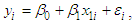 | (5a) |
where  is the error term. The LS estimate of slope
  , the B&G model Energy charge, (see S. Weisberg (2014), p. 24), is given by
 | (6) |
and the LS estimate of the y-intercept  , the B&G model Customer charge, is given by
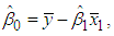 | (7) |
where 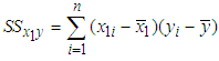 ,
,  Now based on the regression of
  (maximum demand) on
  (energy consumption), which is
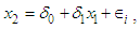 | (7a) |
where  is the error term, the LS estimate for
  is given by
 | (8) |
andthe LS estimate for  is given by
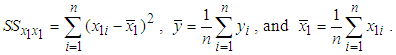
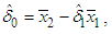 | (9) |
where 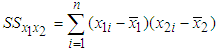 , and
, and  and
and  are as defined earlier. Let us denote the correlation between kWh energy consumption
  and kW maximum demand
  by
by  . The correlation between energy
  and demand
  is computed as, (see S. Weisberg (2014), p. 23)
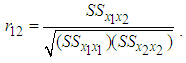 | (10) |
Now we express  given in (8) in terms of the correlation
  given in (10) as follows
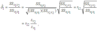 | (11) |
where 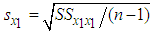 is the standard deviation of kWh energy consumption
  and similarly
 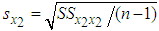 is the standard deviation of kW maximum demand
  From the 3-part CED model (5), the average bill can be computed as
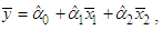 | (12) |
where  , and
, and  and
and  are as defined earlier. Now subtracting equation (12) from equation (5), we get
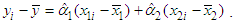 | (13) |
Substituting (13) into the expression 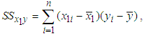 which was used in (6), we get
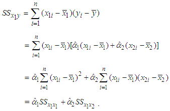 | (14) |
Substituting (14) into equation (6) and using (8), we are able to write  as
as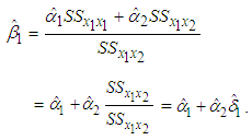 | (15) |
Using equation (11),  (the B&G model’s Energy charge), given by (15) can be rewritten as
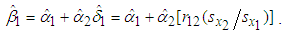 | (16) |
Since the average monthly bills  are the same for both the 3-part CED model and the 2-part B&G model (so both models collect the same amount of dollars), we substitute
  given in (12) into equation (7), and subsequently using equations (16), (11), and (9), we can rewrite the B&G model Customer charge
  as
as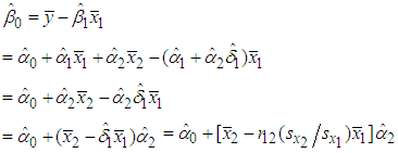 | (17) |
 | (18) |
4.1. Effect of the Correlation between Energy and Demand ( ) on B&G Model Parameters
Below we examine the B&G model parameters in two extreme cases: when  Case I. When
  , the B&G Customer charge
  given in (17) and the B&G Energy charge
  given in (16) take the following form
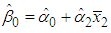 and
and respectively. Under this case, the B&G model takes the form
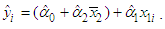 | (19) |
Thus, when there is no correlation between energy consumption and maximum demand, i.e. when  , the B&G model produces an Energy charge that is the same as the Energy charge of the 3-part CED model and all demand-related costs are allocated to the B&G Customer charge.Case II. When
  , then energy consumption
  and maximum demand
  are perfectly linearly related with no error and
  . So, in this case
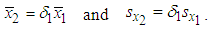 | (20) |
Now using the relationships given in (20), the B&G Customer charge  given in (17) and the B&G Energy charge
  given in (16) take the following form
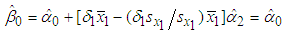 and
and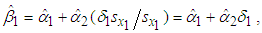 respectively. Under this case, the B&G model takes the form
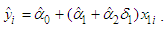 | (21) |
Thus, when there is perfect correlation between energy consumption and maximum demand, i.e. when  , the B&G model produces a Customer charge that is the same as the Customer charge of the 3-part CED model and all demand-related costs are allocated to the B&G Energy charge.
4.2. Allocation of Demand-related Costs between the B&G Customer Charge and the B&G Energy Charge
From the 3-part CED model (5), the average bill can be computed as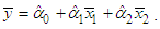 | (23) |
From the 2-part B&G model (5a), the average bill can be computed as | (24) |
Since the average bill in both the 3-part CED model and the 2-part B&G model are the same for the reasons stated above, equations (23) and (24) are equal and we can thus partition the demand-related portion of the average bill,  , from the 3-part CED model as
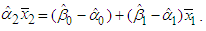 | (25) |
The first term  is the amount of average demand-related costs that will be allocated to the B&G model Customer charge. Similarly, the second term
  is the amount of average demand-related costs that will be allocated to the B&G model average Energy charge.Thus, the proportion of demand-related costs that will be allocated to the B&G Customer charge is given by
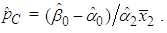 | (26) |
Using equations (9), (11), and (17), equation (26) can be written as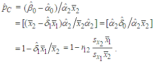 | (27) |
The proportion of demand-related costs that will be allocated to the B&G Energy charge is given by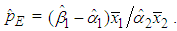 | (28) |
Using equations (11), (16), and (27), equation (28) can be written as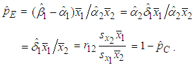 | (29) |
Substituting 0 or 1 for  in equations (27) and (29) produces the same results as in section 4.1 above.When
  , from (27) we get
  and consequently from (29) we get
  . Thus, when there is no correlation between energy consumption and maximum demand, the B&G model allocates all demand-related costs to the Customer charge and allocates no demand-related costs to the Energy charge.Similarly, when
  , from (20) and (29),
  evaluates to
 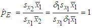 and consequently from (29),
  . Thus, when there is perfect correlation between energy consumption and maximum demand, the B&G model allocates no demand-related costs to the Customer charge and allocates all demand-related costs to the Energy charge.Since
  , the coefficient of variation of maximum demand
  , and
, and  , the coefficient of variation of energy consumption
  , equations (27) and (29) can be rewritten as
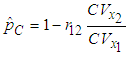 | (29a) |
and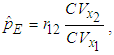 | (29b) |
respectively.
5. The Statistical Data Analysis
The data set used in this analysis includes  individual residential customers’ actual monthly energy consumption (
 ) in kWh, actual monthly maximum demand (
 ) in kW, and calculated monthly 3-part CED bill (
 ) in dollars for the 12 months of August 2016 through July 2017. Although an annual analysis would be a more appropriate procedure for implementing the B&G methodology in practice, we have analyzed each month separately here to illustrate how variations in kWh and kW affect the proportion of demand-related costs allocated to each component of the 2-part B&G rate. Below we discuss only the analysis of data for the month of August, 2016. The results are similar for the remaining 11 months and are shown in the Appendix.The 3-part CED model, equation (5), for this data set is
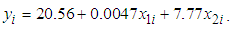 | (30) |
Thus, the CED model Customer charge ($/month) is  , the CED model Energy charge ($/kWh) is
  , and the CED model Demand charge ($/kW) is
  . Here
  represents the ith customer’s calculated CED model bill for the month of August,
  denotes the ith customer’s actual energy consumption (kWh) during the month of August, and
  denotes the ith customer’s actual maximum demand (kW) during the month of August.The estimated August bills
  based on the 2-part B&G model, equation (5a), are the “fitted” regression of calculated bills
  from equation (30) on actual energy consumption
  for the ith customer for the month of August and are
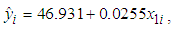 | (31) |
where  is the B&G Customer charge, and
  is the B&G Energy charge. The fitted model in (31) minimizes the sum of the squared deviations between the calculated August bills
  under the 3-part CED model and the fitted August bills
  under the 2-part B&G model.The fitted regression of maximum demand
  on energy consumption
  equation (7a), for this August data is
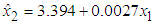 | (32) |
where  and
and  with
with  ,
,  , and
, and  .Now observe from equation (31), (18), and (15) that
 and
and Thus, from the data we observe that our assumed model is appropriate.
5.1. Allocation of Demand-related Costs between the B&G Customer Charge and the B&G Energy Charge
Applying equation (27) to the August data, the proportion of demand-related costs to be allocated to the B&G Customer charge is Applying equation (29) to the August data, the proportion of demand-related costs to be allocated to B&G Energy charge is
  A summary of the 3-part CED model, the 2-part B&G model, and the regression of demand on energy for the month of August are given in Table 1. below.
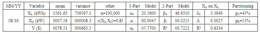 | Table 1. Summary of results for the month of August, 2016 |
The results of the remaining eleven months are listed in Table 2.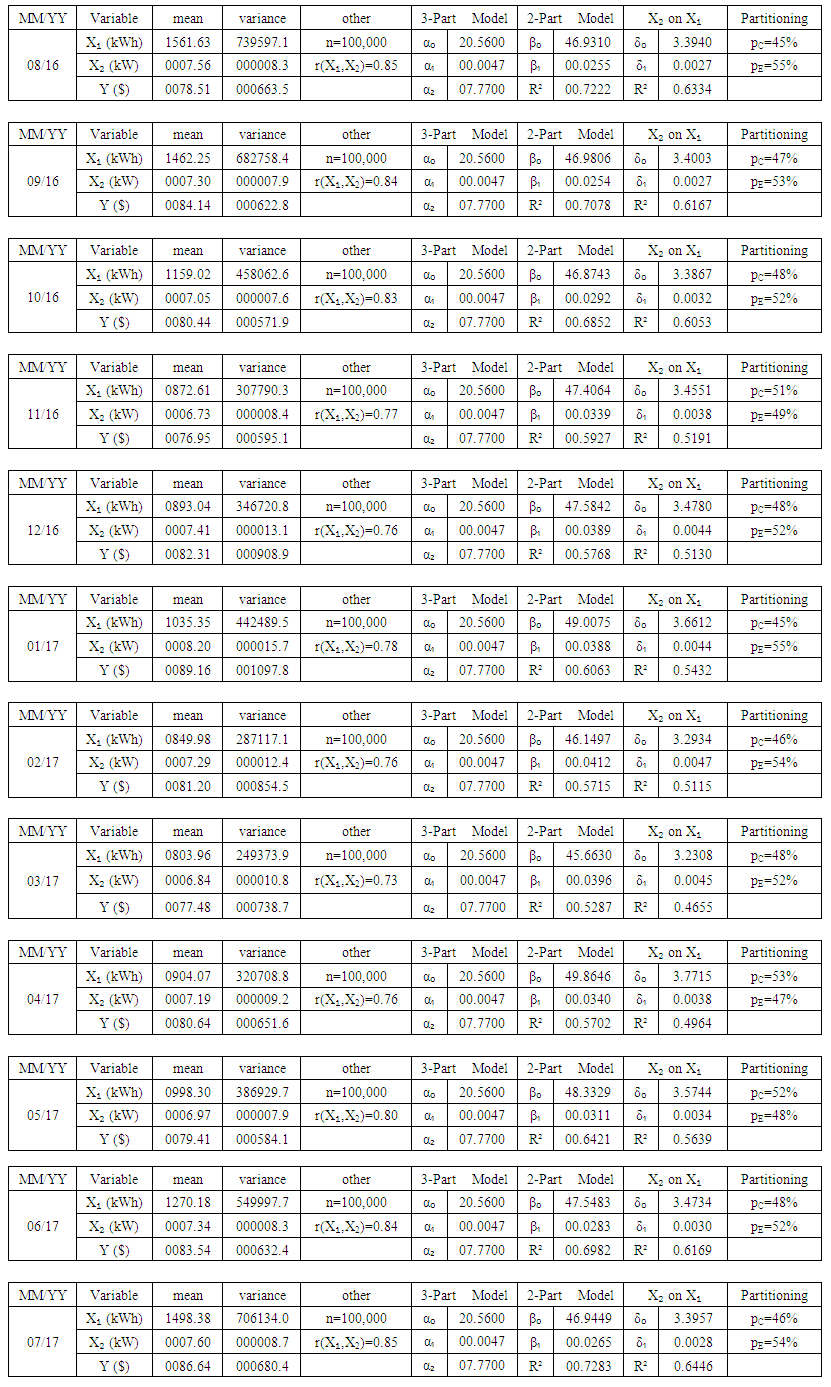 | Table 2. Summary of regression results for all twelve months |
6. Concluding Remarks
This paper further develops the 2014 and 2016 work of Drs. Larry Blank and Douglas Gegax by providing a mathematical description of how energy and demand variations across households affect the proportion of demand-related costs allocated to the two parts of a residential electricity rate using the B&G methodology. Twelve months of actual kWh and kW data for 100,000 residential customers were used to illustrate the mathematical conclusions.As shown in equations (29a) and (29b), the proportion of demand-related costs allocated to each component of the 2-part residential rate depends on the correlation between monthly energy and demand as well as the coefficients of variation of demand and energy. Blank and Gegax (2016) estimated these proportions only empirically. We derived these closed forms theoretically and verified empirically. As evidenced by the mathematical examination in this paper, these factors are fully incorporated in the single linear regression of the B&G methodology.
ACKNOWLEDGEMENTS
The authors gratefully acknowledge the contribution of Mr. Daniel S. Merilatt who first pointed out a mathematical connection between r12 (correlation of kWh to kW) and the proportion of demand-related costs allocated to each component of the 2-part residential rate under the B&G methodology. The authors would also like thank a referee for constructive suggestions on the earlier version.
References
| [1] | Blank, L., and Gegax, D., (2014). Residential Winners and Losers behind the Energy versus Customer Charge Debate. The Electricity Journal 27(4), 31-39. |
| [2] | Blank, L., and Gegax, D., (2016). An enhanced two-part tariff methodology when demand charges are not used. The Electricity Journal 29, 42-47. |
| [3] | Brown, S.J., and Sibley, D.S. (1986). The theory of public utility pricing. Cambridge University Press, Cambridge. |
| [4] | Coase, R.H. (1946). The marginal cost controversy, Economica, 13, 169-189. |
| [5] | Eriksson, R., Kaserman, D. L., and Mayo, J. W., (1998). Targeted and untargeted subsidy schemes: evidence from post-divestiture efforts to promote universal telephone service, J. Law Econ., 41, 477-502. |
| [6] | Weisberg, S., (2014). Applied Regression, 4th edition, Wiley, New Jersey. |

 Abstract
 Reference
 Full-Text PDF
 Full-text HTML