Isaac Ofori Asare1, Dorothy Anima Frempong2, Paul Larbi3
1Mathematics Department, Kwame Nkrumah University of Science and Technology, Ghana
2Computer science Department, Accra Technical University, Ghana
3Kwame Nkrumah University of Science and Technology, Kumasi, Ghana
Correspondence to: Isaac Ofori Asare, Mathematics Department, Kwame Nkrumah University of Science and Technology, Ghana.
| Email: |  |
Copyright © 2018 The Author(s). Published by Scientific & Academic Publishing.
This work is licensed under the Creative Commons Attribution International License (CC BY).
http://creativecommons.org/licenses/by/4.0/

Abstract
Knowing the water level of the Akosombo Dam would help Ghanaian since we depend heavily on hydroelectric power. When the future of the water level is known, society would be able to plan on the usage of electricity for the industries, society, individuals who use some of the water storage for irrigation, water supply purposes. The study employed rainfall from the 12 catchment areas to the River Volta and the daily water level of the dam for a period of 78-years. Principal Component Regression was applied to the input variables for the reduction of its large size to a few principal components to explain the variations in the original dataset. The outcome of the PCR extraction was two principal components. Time Series using Seasonal Autoregressive Integrated Moving Average was used to model the data. The appropriate model that fit the data well was ARIMA (2,1,2) (1,0,0) [12] after comparing other models AICs. The model with the smallest AIC and the least number of parameters was selected as the best model.
Keywords:
Principal Component Regression, Time series, ARIMA, SARIMA, Measures of Adequacy
Cite this paper: Isaac Ofori Asare, Dorothy Anima Frempong, Paul Larbi, Use of Principal Components Regression and Time-Series Analysis to Predict the Water Level of the Akosombo Dam Level, International Journal of Statistics and Applications, Vol. 8 No. 6, 2018, pp. 332-340. doi: 10.5923/j.statistics.20180806.07.
1. Introduction
The hydroelectric project is a physical structure constructed for the generation of hydropower. They have been used as a structural mechanism to regulate the flow of water for storages purposes. The structure (hydro project) are made to reduce the fast flow of water to the dam. The hydroelectric projects are capable of storing flow of rainwater to ensure water supply for hydro-power generation and for other economic purposes such as for agro-business, household and industry usage. During raining season, the dam is able to get enough water for it intended purposes, production of enough hydropower. When there is drought, the water level of the dam reduces which limit the production of electricity as Ghanaians depend largely on hydropower for domestic and industrial usage. The dam level depends largely on rainfall from some catchment's areas of Ghana. When it rains in these areas the water flow into the tributaries and then move to the river Volta. There is the need to know the contribution of each of these catchment areas when it rains and their impact on the water level of the Akosombo dam. Also, as a major source of hydro-power, there is the need to be able to forecast the water level at a time accurately and precisely to determine the amount of energy that might be produced at a particular point in time, daily, weekly, monthly or even yearly. A result of that there was the need to have good forecasting tool that could help forecast the water level of the dam accurately and precisely.At the beginning of the year 2007, Ghanaians were worried and raised concerns about the limited hydro-power generation (electricity) or supply from the generation plant (dam) due to the low water levels in the Lake Volta reservoir, reports from the dam site indicating that the project was functioning below its capacity due to the problems of drought due to global warming. It implies that when there is minuscule or no rains from the river catchment areas to feed it, the Akosombo dam level would be low and as a result, the dam would not be able to perform up to expectation.In the year 2010, the country experienced high rains and as a result, the Akosombo dam site recorded the highest water level due to heavy rainfalls in a catchment area contributing to the dam, the reservoir elevation went above it expected a value of 84.73 m (278.0 ft). Due to the raised in the water level of the dam, it caused management of the dam site to let some of the water flow out by allowing some of the water to pass through the floodgates at a basin elevation of 84.45 m (277 ft), and for several days, weeks, water was still spattering from the river, creating some flooding in the nearby communities along the dam site.According to the Ghanaian times on June 7, 2016, at the time when the report has been filed, the dam level of the reservoir was approximately 237.27 ft, just a little below the 240 ft the accepted level that can enhance the operation of the plant a situation the VRA has been threatened with all this while. The Corporate Affairs Manager at the VRA, Mrs Getrude N. Koomson, in a formal interview with one of the new papers; the Ghanaian Times indicated that the situation was causing the machinery to underperform.This news indicates that until the water level appreciates to up to certain level to empower all the six turbines run concurrently, then the alternative they would be left with was to relying on or cope with the little inflow and to ensure that the engineers keep at most four of the turbines running subject to the demand of hydro-power in the country (Ghana). This is as a result of low rainfalls in the country. When there are rains from the catchment areas especially the medium or the central belt and the northern zones of the country. The situation the dam is experiencing could change if there are rains from these areas.The water level of the dam is mainly for hydropower and other purposes such as water storage which has been employed for irrigation needs and water supply for domestic use are some key importance of the dam, therefore there is the need to knowing the water level of the dam for effective and efficient planning and the need to knowing the contributions water from the various catchment areas to the dam for the desired performance. This could be done when we know the main contribution of the various catchment areas to the water level in the dam and based on it the forecasting techniques can be employed to ensure effective and accurate result when we know the contribution of water by the catchment areas can be obtained. There are factors that influence the water level negatively such as evaporation, soil moisture and human activities along the banks of the river, these are factors that need to be considered in forecasting of the water level. Marino et al (2017) climate change can cause the distribution of rainfall patterns, with potential effect for the water bodies. Changes in water bodies' level are as a result of factors such as like rains and other atmospheric conditions such as temperature, evaporation and humidity. When there is continuous wet and cold condition over a period of time, the volume of water levels rises, on the contrary, warm and dry periods would cause the water levels to decline. The global warming can affect the normal cycle of rainfall, thereby destroying the water supply and demand and having a significant impact on water bodies, agriculture, human health, animals and plant, this condition could prolong drought and water shortages (Brebbia, 2011).
2. Research Problem
The Akosombo Hydroelectric Project requires rainfalls from its catchment areas to operate effectively for generating of hydroelectric power and production of water for domestic consumption and industrial usage to Ghanaians and other nearby countries. According to the Ghana Metro-logical Agency, the Akosombo Dam takes its volume of water from about 12 catchment areas (stations) when it rains in these areas, therefore contribute significantly to the water level of the dam. They are as follows; Kintampo, Bui, Tamale, Yendi, Akuse, Navrongo, Salaga, Kate-Karachi, Bole, Atebubu, Kpando and Ho. Ghana depends so much on the Akosombo Hydroelectric power for its activities there is the need to get a model that can improve the older models used in predicting the water level. The study adopted Principal Component analysis to reduce these rainfall stations to few stations that could be used to describe the variation explained by all the stations. Though the traditional time series model does not consider nonlinear inputs, hence giving out inconsistency results in its anticipation as indicated by Rani and Parekh (2014). The traditional time series technique is efficient and effective for a long time, but there was a deficiency that they suffer that is the issue of stationary and linearity. Though the ARIMA model does not take into consideration nonlinear data, the process of transformation could be applied to the data to make it linearize. Also differencing could be applied to the data if the dataset is non-stationary to make it stationary. Ghana depends heavily on hydropower (Akosombo) for electricity, there is the need to get model that could be used to forecast the water level of the Akosombo Dam at any given time been daily, monthly or year based for proper planning of the power issues in the country. Planning for the hydroelectric project is a very essential step for success in the evolution of Ghana since we depend mainly on hydro-power. This progress would be successful if the water level of the dam is determined correctly or checking for accuracy of the dam water level. As a result of this prediction; the study adopted Principle Component Regression (PCR) and variable importance using the random forest technique in the determination of the important rainfall catchment area having an impact on the water level.
3. Specific Objectives of the Study
1. Knowing the impact of rainfall basin stations in terms of percentage to the Akosombo Water level. 2. Reduce the number of rainfall basins stations contributing to the Akosombo water level to a few Principal Components.3. Get a good forecast technique for the water level of the Akosombo Dam.
4. Research Methodology
The Akosombo hydroelectric project is greatly influenced by several atmospheric conditions or atmospheric factors such as rainfalls, the flow of water sources, warmth and high temperature, and even heat due to evaporation or humidity. Due to the unavailability of data on the side of the researcher, the study focused on upstream rains and past data on the dam level. The data used for the research were the past rainfalls monthly for a period of 78years making 948 data point from the 12 major tributaries of the Volta River from 1936-2014. They include; Kintampo, Tamale, Bui, Yendi, Navrongo, Salage, Kata-Krachi, Bole, Atebubu, Kpando, Ho and Akuse stations. Also, monthly data on the water level of the Akosombo Dam was obtained. The principal component was applied to these stations in determining the most significant stations that could be used to explain the variation in the water level when it rained over these stations. 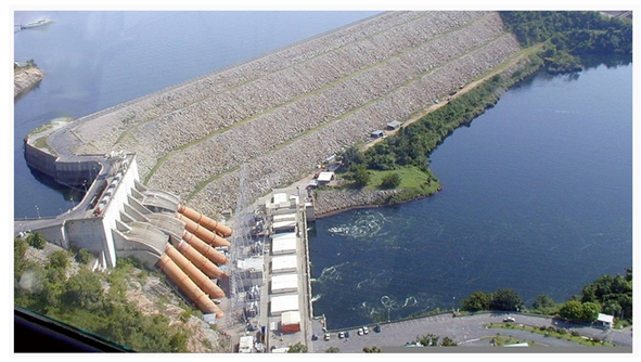 | Figure 1. Akosombo Dam water level |
5. Model Specification
Principal Component Regression and Random Forest techniques were used to analyse the data gathered. perform principal components analysis (PCA) was performed first on the on the original data, then perform dimension reduction by selecting the number of principal components (m) using cross-validation or test set error, and finally conduct regression using the first m dimension reduced principal components.
6. Multicollinearity: Examination of Correlation Matrix
One of the assumption underlings the usage of PCA /PCR is to ensure that, there is independency among the variables. There would be the independence of the variables when there is no multiclonality among the variables. A high value of the correlation between two variables may indicate that the variables are collinear. This method is easy, but it cannot produce a clear estimate of the degree of multicollinearity. (El-Dereny and Rashwan, 2011). The correlation coefficients are greater than 0.80 or 0.90 then this is an indication of multicollinearity. Variance Inflation Factor (VIF) is one of the techniques that is used to assess the level of collinearity in an ordinary least square regression analysis. if any of the VIF values exceed 5 or 10, it is an indication that the associated regression coefficients are poorly estimated because of multicollinearity (Montgomery, 2001). The VIF is calculated as | (1) |
where  represent the coefficient of determination when
  is regressed on all other predictor variables in the model.
7. Eigen Analysis of Correlation Matrix
The eigenvalues can also be used to measure or determine the component the number of components that have to be extracted. It can check for the presence of multicollinearity in the predictor variables, one or more of the eigenvalues will be small (near to zero).
8. Principal Component Regression (PCR)
The PCR is used to handle multicollinearity among variables, it is not usually included in standard regression analysis. The PCA follows from the fact that every linear regression model can be restated in terms of a set of orthogonal explanatory variables. These new variables are obtained as linear combinations of the original explanatory variables. They are referred to as the principal components. The independent variables in the PCR are given as; | (2) |
Where  is the ith observation on the jth variable, and
  and
and  represent the estimated mean and standard deviation respectively. The dependent variable is cantered;
  | (3) |
The transform matrix  , where X is the
  matrix of
  observations on p independent variables, Z is the
  matix of transformed data whilst A is the
  matrix consisting of eigenvectors. The regression model is given as;
 | (4) |
where B is the px1 vector of unknown parameters and it is estimated as;  | (5) |
The regression equation for the PCA is given as;  | (6) |
9. Time Series Statistical Models
The Box -Jenkins methodology was duly followed in the estimating of the parameters in the time series analysis (Box and Jenkins, 1970). The Auto-regressive and the Moving Average (ARMA (p, q)), or Auto-regressive Integrated Moving Average (ARIMA (p, d, q)) was adopted for the prediction of the time series data. Nevertheless, the application of the ARMA model assumes that the time series data be stationary; which implies, ARMA processes remains in the stability about a constant mean level. However, when data are nonstationary or have obvious trend variability, the ARIMA model built on the differencing algorithm could be adopted (Box et al. 1994). The Augmented Dickey-Fuller (ADF) is used to examine for the stationarity in the dataset test (Elliott et al. 1996).
10. Measures of Adequacy
The following measures of adequacy were used to test for the adequacy of the time series model. The performance of the proposed time series is assessed with these criteria; Mean Absolute Error (MAE), Mean Absolute Percentage Error (MAPE), and Root Mean Square Error (RMSE) and Mean Square Error (MSE).Let  represent the
  observations and
  denote the forecast, where
  the adequacy measures are as follows;
 | (7) |
 | (8) |
 | (9) |
 | (10) |
11. Results
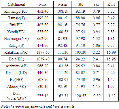
The results in the table below show the descriptive statistics of the monthly rainfall of the 12 tributaries of the Akosombo dam water level of the Akosombo Dam for a period of 78 years, ranging from 1936-2014. The minimum rainfall for all the various tributaries was zero (0) meaning that there were no rains in such area in the case of the water level, the zero value means that the water level record was not captured for a reason not made available to the researcher. The maximum rainfall for all the 12 tributaries is shown in the table. The average rainfall for Kintampo is 108.188 with a deviation of 92.186, Tamale has a mean rainfall of 90.154 and a deviation of 88.979. Bui has an average rainfall of 94.161 and a deviation of 76.757. The results show that a rainfall in Kate-Krachi and Bole were not normally distributed. Since the skewness and the kurtosis for each of them was above ± 1.96. The rest of the rains from the catchment areas were normally distributed.Table 1. Descriptive statistics of the variables
 |
| |
|
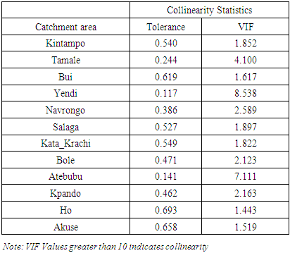
Table 2. Diagnostics analysis
 |
| |
|
Collinearity diagnostics was performed and the results obtained shows that none of the catchment areas has more than 10 Variance Inflation Factor (VIF). The least VIF value is 1.443 associated with Ho and the maximum VIF is 8.538 also associated with Yendi. This means that there is no problem of multicollinearity.Once there is no problem of collinearity among the independent variables, the data gathered was standardize first to ensure that each predictor is on the same scale as the other variable. This is done to prevent the algorithm to be skewed towards predictors that are dominant in absolute scale.
12. Principal Component Analysis Results
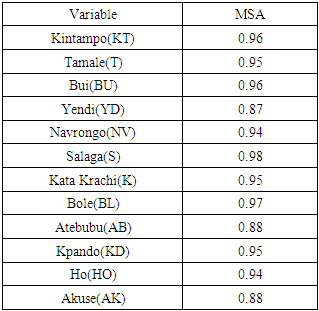
The results in the table below shows the Measures of Sampling Adequacy (MSA), though the MSA does not produce or show the p-values to determine the significance of the results, however MSA value of at least 0.80 is considered acceptable in terms of the sample adequacy used for the study as indicated by Norman & Streiner (2008). The analysis of the results shows as shown in Table 3 below shows the MSA for the variables used for the study. The results in the table show that the least MSA is that the least MSA is 0.87 which is associated with rains from Yendi and the highest MSA being 0.98 which is also associated with Salaga.Table 3. Anti-image Correlation
 |
| |
|
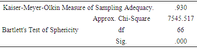
The Bartlett Test of Sphericity which was used to compares the correlation matrix with a matrix of zero correlations usually known as an identity matrix, which consists of all zeros except the 1's along the leading diagonal. The results obtained shows that, factor analysis is appropriate to fit the data gathered due to high MSA and also a significant Bartlett’s Test of Sphericity value of p-value <0.001 at 5% significance level. However, the overall KMO value of 0.930 indicates that the sample size used for the study is adequate.Table 4. KMO and Bartlett's Test
 |
| |
|
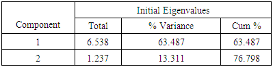
The results from the principal components analysis show that there are two main components extracted from the from the 12 tributaries that contribute to the Akosombo water level. The Total variance explained which indicates how much of the variability in the data has been explained by the components is shown in table 3 below. From the analysis, the first component has an eigenvalue of 6.538 and a variance of 54.487%. The second components have an eigenvalue of 1.237 and a variance of 10.311%. The results of the components had an eigenvalue less than 1. Cumulatively the two components could explain about 76.798%. This means that the water level from the various tributaries can be clustered into two main groups. The figure 2 below shows the scree plot of the number of principal components that were extracted showing the components eigenvalues. Kaiser (1970) component that has an eigenvalue of at least one was extracted which is what is shown in the figure below.Table 5. Total Variance Explained
 |
| |
|
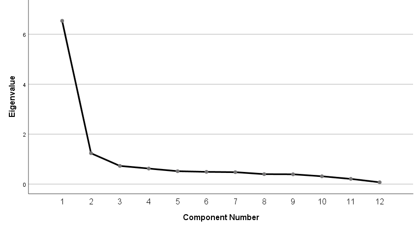 | Figure 2. Scree Plot |
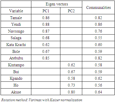
In this research work, two components were extracted as indicated in the figure above cutting off after component 2. This shows only two components were extracted work. The two principal components could explain about 76.798% as indicated in table 5 above.Table 6. Results of PCA (Varimax Rotated Matrix)
 |
| |
|
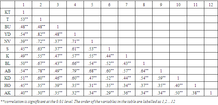
The results in Table 6 above shows the Varimax rotation for the components model along with their communalities. The results for the rotation are quite comparable and easy to interprets. Two main components were extracted to represent the 12 components it shows that, seven (7) main variables correlate well with component 1 and among the eight variables, Yendi and Navrongo highly correlate well with component 1. Also, four (4) variables correlate well with the second component. A threshold of 0.60 was used for identifying a reliable factor in this study as indicated by (Stevens, 1996). Hair et.al (2010) indicated that items that load less than 0.50 are not accepted. From the results in table 6, only one variable had a loading of less than 0.60, the rest are having significant loadings above 0.60. There was no problem of cross-loadings between the variables all the variables have loadings or more than 0.60. This means that more than one-half of the variations in the dataset are accounted for by the loadings on a single factor. Factor loadings (<0.50) have not been shown and the results have been sorted by loadings on a particular component. The result in table 7 below shows the Pearson bivariate correlation between the standardised of the variables used for the study. Tabachnick and Fidell (2001) indicated that the correlation between variables less than 0.30 is not appropriate for exploratory analysis and from the result obtained as indicated in table 7, below. From the table, there is no such problem. El-Dereny and Rashwan (2011) indicated that the correlation between variables which results in rho  of more than 0.80 is also not appropriate for exploratory analysis. The results obtained indicate that there is none of such problem. The minimum correlation value obtained is rho
  whilst the maximum correlation value rho
  Those these values were either below or above the accepted range of values their impact is insignificant since it only occurred between two sets of variables, between Akuse and Salaga (
 and between Tamale and Yendi
  The results suggest that the variables are not much correlated hence there is the independence of the variables in the model.
 Table 7. Bivariate Correlation Analysis
 |
| |
|
13. The Principal Component Regression (PCR)
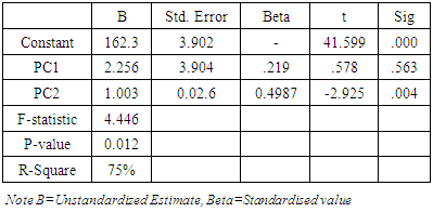
After the extraction of the two main components, the eigenvectors for the two components were used as regressors for the regression analysis and the results show that there is at least a significant component in the model. The f-statistics was statistically significant at 5% significance level (F=4.446, p-value=0.012). Also, the R-square was approximately 75% to show how much the components can be explained on the dependent variable. The estimated PCR that fits the data gathered is given as; | (11) |
Table 8. Coefficients of the PCR
 |
| |
|
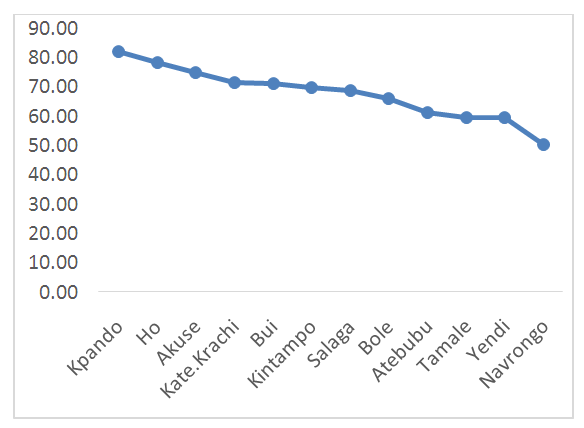 | Figure 3. Variable importance (Mean Decrease Gini) |
Variable importance test was performed on the data using random forest and the result obtained indicates that rainfall from the catchment area(s) are statistically significant havig impact on the water level of the dam. From the figure 3, it could be observed that, among the 12 rainfall catchment areas, rains from Kpando is the most important area having an impact on the Akosombo water level, followed by rains Ho, Akuse, Bui and then Kate-Krachi among others as shown in the figure above. Also, figure 4 shows the multiple plot of all the rainfall catchment areas. The Geni value for Kpando is estimated to be 81.97, Ho value is 77.23, Akuse is 75.20, Kata Krachi is 70.61 among others as shown in the figure below.The results in figure 4 below show the multiple plots of the rainfall recorded for a period of 78 years from the twelve (12) catchment areas.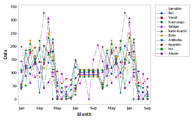 | Figure 4. Multiple time plot of the 12 tributaries of the Akosombo water level |
14. Seasonal Autoregressive Integrated Moving Average (SARIMA)
Time series analysis was carried on the monthly water level of the dam for the period of 78years. The initial plot of the data shows that there is some level of fluctuation in the dataset. The stationary test was performed and the results show that the dataset s stationary at 5% significance level with Augmented Dickey-Fuller Test value of -5.0468, Lag order=8, p-value=0.01. 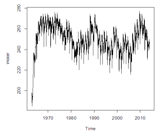 | Figure 5. Time series plot of water level |
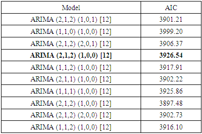
The plot shows some seasonal component and as a result, the appropriate model was selected based on the model with the least AIC. The selected model to fit the data is Seasonal Autoregressive Integrated Moving Average (SARIMA) and from the analysis, the results show that the appropriate model to fit the data gathered is ARIMA (2,1,2) (1,0,0) [12] as indicated in table 9 below. Table 9. Selection of best model
 |
| |
|
15. Significance of Coefficients
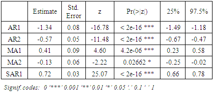
The result of the selected best model has the following coefficient value with their confidence interval at 25% and 97.50%. The results show that the estimated AR1 value is -1.34, with a standard error of 0.08 and a small p-value less than 0.05. AR2 has -0.57 coefficient value and a small p-value less than 0.50. The MA1 component has an estimated value of 0.41, with an error margin of 0.09 and a small p-value of less than 0.5. The MA2 has a coefficient value of -0.13 and a small p-value. However, the seasonal component of the model, SAR1 has an estimated value of 0.72 with an error margin of 0.03 and a small p-value. The result indicates that all coefficients are statistically significant.Table 10. Coefficient estimate
 |
| |
|
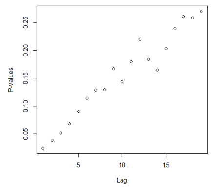 | Figure 6. Ljung-Box Q Test |
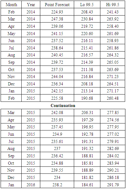
The residual of the model was tested and the results obtained shows the p-value for the Ljung-Box Q test all are well above 0.05, indicating non-significance and this an indication of good and desirable result.Table 11. Forecast value for the 24months
 |
| |
|
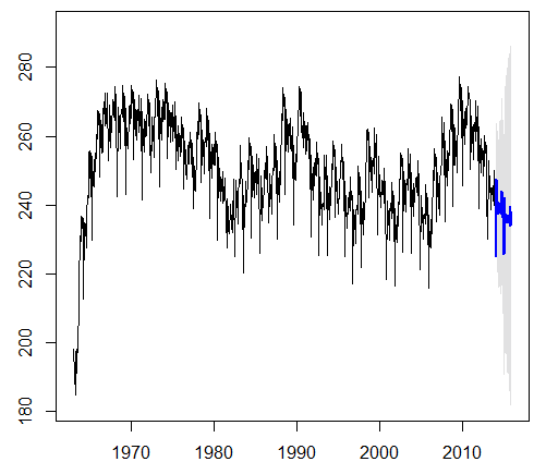 | Figure 7. ARIMA (2,1,2) (1,0,0) [12] |
The results in Table 11 depict the forecast value of the next 2years (24 months). The estimation was done with a 99.5% confidence level (lower and the upper confidence level) and figure 7 above shows the diagrammatical representation of the forecast values for the period of 24 months. The forecasts are shown as a blue line, with the 80% prediction intervals as a dark shaded area, and the 95% prediction intervals as a lightly shaded area as indicated in the table 6 above.
16. Conclusions
In this work, the Principal component analysis was used to classify the tributaries of the Akosombo water level into two main components (PC1 & PC2). The variances that were explained by the two components was 76.798% as indicated in the table above. The approach presented here is efficient and appropriate for classification of water level that makes up the Akosombo water level. After the classification, the eigenvectors were regressed on the water level and the results show that PC2 has a significant impact on the water level. This means that, when there are more rains in these catchment areas such as Kintampo, Bui, Kpando, Ho and Akuse, it will have a significant impact on the Akosombo water level. The impact of rains from these catchment areas is approximately 50% and whilst the PC2 has about 22% impact on the dependent variables as indicated in the table above. The estimated RMSE value of the model was 7.07, MAE=4.89, MPE=0.11, MAPE=1.97. The best model was estimated to be; ARIMA (2,1,2) (1,0,0) [12] with an overall AIC value of 3926.54.
17. Recommendations
Further studies must be done to improve upon the results of this study, by considering factors such as accurate prediction of the water level of the dam at any time using other modelling technique such as the Artificial Neural Networks, since most researchers have used it in modelling water resources data. Prediction for a period of 2years (24 months) was estimated at a 99.5% confidence level.
18. Limitation of the Study
This study made use of the rainfall from the river basins areas for its prediction, due to the lack of data on other variables for predictions. For accurate and precise prediction of the water level of the dam, factors such as temperature, humidity and the flow rate of the water from the main tributaries of the river Volta must be included, because these variables have got much impact on the water level. Also, further studies could be done to improve upon the prediction level of the ARIMA (2,1,2) (1,0,0) [12] by the use of Artificial neural networks.
ACKNOWLEDGEMENTS
We are very grateful to the staff of the Akosombo Engineering Department (Akosombo Dam Site) for their contribution towards this study.
References
| [1] | Box, G.E.P. and G.M. Jenkins (1970). Time Series Analysis, Forecasting, and Control. Oakland, CA: Holden-Day. |
| [2] | El-Dereny, M., & Rashwan, N. I. (2011). Solving multicollinearity problem using ridge regression models. Int. J. Contemp. Math. Sciences, 6(12), 585-600. |
| [3] | Elliott, G., Rothenberg, T. J. and Stock, J. H. (1996). `Efficient Tests for an Autoregressive Unit Root', Econometrica, 64, 813-836. |
| [4] | Hair, J. F., Anderson, R. E., Tatham, R. L., & Black, W. C. (1995). Multivariate data analysis with readings (4th ed). New Jersey: Prentice-Hall International. |
| [5] | Hair, J. F., Black, B., Babin, B., Anderson, R. E. and Tatham, R. L. (2010). Multivariate Data Analysis: A Global Perspective. Pearson Education Inc., NJ. |
| [6] | Kaiser, H. F. (1970), “A Second-Generation Little Jiffy,” Psychometrika, 35, 401–415. |
| [7] | Marino, N. A., Srivastava, D. S., MacDonald, A. A. M., Leal, J. S., Campos, A. B., & Farjalla, V. F. (2017). Rainfall and hydrological stability alter the impact of top predators on food web structure and function. Global change biology, 23(2), 673-685. |
| [8] | Montgomery DC, Runger GC (1999). Applied statistics and probability for engineers. Wiley, New York. |
| [9] | Norman, G. R., & Streiner, D. L. (2008). Biostatistics: the bare essentials. PMPH-USA. |
| [10] | Rani, S., & Parekh, F. (2014). Predicting reservoir water level using artificial neural network. International Journal of Innovative Research in Science, Engineering and Technology, 3(7), 14489-14496. |
| [11] | Stevens, J. (2001). Applied Multivariate Statistics for the Social Sciences; Lawrence Erlbaum: Mahwah, NJ, USA, 1996. |
| [12] | Tabachnick, B. G., & Fidell, L. S. (2001). Cleaning up your act: Screening data prior to analysis. Using multivariate statistics, 5, 61-116. |
| [13] | https://en.wikipedia.org/wiki/Volta_River. |
| [14] | http://www.ghanaiantimes.com.gh/akosombo-dam-level-drops/ |

 Abstract
 Reference
 Full-Text PDF
 Full-text HTML