Mossamet Kamrun Nesa
Department of Statistics, Shahjalal University of Science and Technology, Sylhet, Bangladesh
Correspondence to: Mossamet Kamrun Nesa, Department of Statistics, Shahjalal University of Science and Technology, Sylhet, Bangladesh.
| Email: |  |
Copyright © 2018 The Author(s). Published by Scientific & Academic Publishing.
This work is licensed under the Creative Commons Attribution International License (CC BY).
http://creativecommons.org/licenses/by/4.0/

Abstract
In order to improve the overall health condition of a population, accurate estimates of health indicators are required at very small spatial scale, typically the administrative units of a country and/or a region within a country. Direct estimation methods tend to have unacceptably high standard errors when the area-specific sample sizes are not large enough. In such situations, model-based small area estimation methods can be conducted based on either area level or unit level models on the basis of data availability and achieve lower mean squared errors. When unit level data are inaccessible, area level models such as Fay-Herriot model have been widely used instead. This paper is concerned with the use of a multivariate Fay-Herriot area level model to get improved estimates for each variable by area rather than using single variable. A simulation study is carried out to investigate multivariate and univariate small area estimators. An empirical study has been performed to compare univariate and multivariate estimators using data from the Bangladesh Demographic Health Survey (BDHS) 2011 and Population Census 2011. In Bangladesh, a few works have been done to estimate district level child nutrition status. The prevalence of nutrition status is assessed by two standard anthropometric indicators: underweight and stunting. Small area estimates of underweight and stunting are calculated from BDHS 2011 with auxiliary variables derived from the Bangladesh Population and Housing Census 2011. The survey Bangladesh DHS covers all districts but district wise sample sizes are very small to get consistent estimates. So Fay-Herriot Model has been used to calculate district wise estimates with efficient mean squared error.
Keywords:
Small Area Estimation, Univariate Fay-Herriot Model, Bivariate Fay-Herriot Model, Relative Efficiency
Cite this paper: Mossamet Kamrun Nesa, Numerical and Empirical Evaluation of Fay-Herriot Models, International Journal of Statistics and Applications, Vol. 8 No. 6, 2018, pp. 291-296. doi: 10.5923/j.statistics.20180806.01.
1. Introduction
Survey data are now widely used to provide estimates not only for the total population but also for subpopulation (also known as domains). Domains can be defined by geographic areas or socio-demographic groups. A domain or area is known as large when the domain-specific sample size is large [1]. Domains or area estimators that are obtained based only on the sample data from the domain or area are known as direct estimators. Direct estimation methods such as the design-based Horvitz-Thompson estimator (HT) [2] or the model-assisted generalized regression (GREG) estimator [3] are effective when the domain-specific sample sizes are large. However, in practice, when the domain-specific sample sizes are not large enough (known as small areas), sufficiently precise direct estimates cannot be produced. In such situations, small area estimation (SAE) methods can be used to get reliable estimates of the parameters of interest from the related areas [4].The basic idea of small area estimation method is to link the variable of interest with auxiliary information (e.g., Census and Administrative data) in a random effects model [5]. SAE method is broadly classified into two methods - Unit level SAE and Area level SAE. When unit level survey data is not available, area level SAE is utilized for small area estimates. One of the basic area level models is the Fay-Herriot (FH) model [6] which relates small area direct survey estimates to area specific covariates. When multiple dependent variables are considered correlated, multivariate Fay-Herriot model may produce better results than univariate FH model [1] but these models have received relatively little attention.Statisticians use the univariate Fay-Herriot (UFH) model for one variable or separately for each variable. However, in some surveys it may be desirable to consider two or more correlated response variables together. In such cases, the multivariate Fay-Herriot (MFH) model can be used to incorporate the correlation among the response variables [7]. When multiple dependent variables are correlated, MFH models may produce better results than UFH models, but these models have received relatively little attention. There is limited work on the benefits of MFH models. More precise SAEs are obtainable using MFH models rather than using separate UFH models for each variable [8]. A simulation study conducted by [9], designed for comparing MFH and UFH estimators, and concluded that multivariate modelling reduced the MSE of the SAE estimators. The focus of this paper is to elucidate how bivariate Fay-Herriot (BFH) models work better than separate UFH models based on MSE. Some special cases are explained which will give insight into when BFH should be worthwhile in practice. A simulation and an empirical study are conducted to compare the two methods. In the simulation study, the behaviour of the UFH and BFH estimators is investigated by generating datasets following [9]. Both the UFH and BFH models are fitted and MSEs of the corresponding empirical best linear unbiased predictor (EBLUP) are calculated using the estimated parameters from the simulated data. In the empirical study, BFH and UFH estimators and the MSE estimator are applied to data from the Bangladesh Demographic and Health Survey 2011 and Bangladesh Population and Housing Census 2011. In Bangladesh, no works have been done to estimate district level child nutrition status either direct or indirect approach. The recent Bangladesh Demographic and Health Survey 2011 covers all districts but district wise sample sizes are very small (10-100) to get consistent estimates [10]. The purpose of this paper is to develop an area level Fay-Herriot Model to calculate district level estimates with their efficiency. Comparison between univariate and multivariate FH models has also been done. The paper is organized as follows: Section 2 outlines the model structure and the MSE for both the UFH and BFH estimators. The relative performance of UFH and BFH estimators is measured by the relative efficiency of these MSEs. Section 3 explain the special cases. Section 4 investigates the performance of the UFH and the BFH estimators via a simulation experiment. Section 5 describes the empirical study and Section 6 summarises the findings.
2. Univariate and Bivariate Fay-Herriot Estimators
The purpose of this section is to make simple comparisons of the MSEs of the BFH and UFH estimators assuming known model parameters including variance components and regression coefficients. However, in practice these parameters are unknown and this must be reflected in MSE estimation when FH estimators are calculated in practice.
2.1. Univariate Fay-Herriot Model
Let  where
where  is the small area mean for the dth area. Suppose
  is related to the auxiliary data
 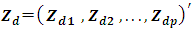 through the model called the linking model:
 The direct estimators of
  follow a sampling model,
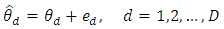 Combining the above two assumptions, the univariate Fay-Herriot model is
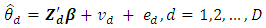 | (1) |
where D is the number of areas,  is a (p × 1) vector of auxiliary variables, and β is a (p × 1) vector of regression coefficients. Furthermore, vd and ed are area specific random effects and sampling errors respectively, assumed to be independent with
 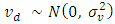 and
and 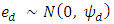 respectively. The disturbance terms
  and
and  are assumed to be independent from each other. Their respective variances,
  and
and  are the area-specific random effect variance and the design-based sampling variance. The BLUP estimator of
  , denoted by
  for known β, is
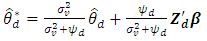 | (2) |
The MSE of the BLUP estimator of,  , is
, is 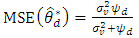 | (3) |
The log-likelihood function of the data  is
is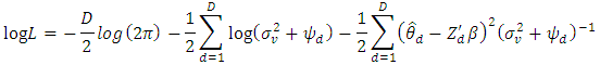
2.2. Bivariate Fay-Herriot Model
Let  be the (2 × 1) vector of the small area statistics in area d for the two target variables. The linking model is
 | (5) |
where  is a (p × 1) vector of auxiliary variables, β is a (p × 2) matrix of regression coefficients and vd are the area specific random effects with mean zero and variance-covariance matrix
  given by:
 where
where  and
and  are the random effects variances of the first and second variables respectively and
  is the random effects covariance term. The direct estimator of
  follows a sampling model,
 | (6) |
where 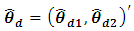 are the direct estimates of
  . Let
. Let  be the sampling error with mean zero and variance–covariance matrix
  where
where  and
and  are the sampling error variances of the estimate of first and second variables respectively with covariance term
  . Combining (5) and (6), the bivariate Fay-Herriot model is
 | (7) |
The BLUP estimator of  for known
  is
is | (8) |
where 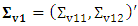 and
and 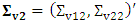 . The BLUP estimator (8) can be written as
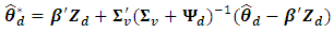 | (9) |
See [1] who derive the BLUP when  is unknown. The MSE of the BLUP estimator of
  is
is | (10) |
which can be expressed as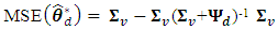 | (11) |
The log likelihood function is
2.3. Relative Efficiency of UFH and BFH Estimators
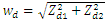
The relative efficiency, RE, of the bivariate BLUP estimator compared to the univariate BLUP estimator is 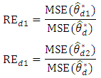 Substituting the expressions of
  and
and  from (3) and (10), the approximate relative efficiencies of the bivariate BLUP estimator compared to the univariate BLUP estimator are
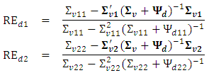
3. Special Cases
When the correlation exists between the response variables, the multivariate model leads to more efficient estimators compared to those based on univariate model [1]. This implies that relative efficiency becomes one the correlation between the sampling errors and random effects for each variable are both zero. In addition, when the sampling errors are zero, then the relative efficiency also becomes zero. It can also be shown that when the covariance term of the random effects is equal to its variance term of the first variable and when the covariance term of the sampling errors is equal to its variance term of the first variable then there is no gain for the first variable. Similarly, when the covariance term of the random effects is equal to its variance term of the second variable and when the covariance term of the sampling errors is equal to its variance term of the second variable then there is no gain for the second variable. However, when the ratio of the variances of random effects is large, there would be some gains of using BFH estimators. These special cases are informative but of course none of them will hold exactly in practice, so a simulation study will be conducted next section to evaluate the relative efficiencies of UFH and BFH estimators.
4. Simulation Experiment
4.1. Design of the Experiment
This section describes a simulation experiment for analyzing and comparing the relative efficiency of small area estimates from the BFH model compared to the UFH model. The simulation follows [9]. Let us consider two response vectors 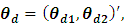 d = 1, 2. . . D, which are assumed to be linearly related to the values of the two explanatory variables. For the simulation study we have D=100 areas. The steps of simulation study are: 1. The values of the explanatory variables
 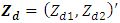 are generated from a multivariate normal distribution as
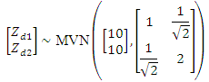 The random area effects
  are generated from a normal distribution with zero mean and unit variance, and the vectors of sampling errors
  are generated from a multivariate normal distribution with mean zero and covariance matrix
 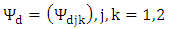 where
where 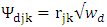 and
and  are the heteroscedasticity weights. For generating
  assume
 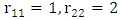 and
and 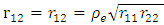 with the heteroscedasticity weights
 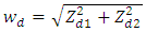 . Two options are implemented here: firstly considering heteroscedasticity weights as
  (homoscedastic model) and secondly heteroscedasticity weights as
 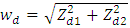 (heteroscedastic model). Like [9], the regression coefficients are set as
  . 2. Using the simulated values of explanatory variables, the random effects and sampling errors, the two response variables are generated with different values of
  via the BFH model (9). 3. Both the UFH and BFH models are fitted to the direct estimates on the explanatory variables using the maximum likelihood (ML) estimation method. ML estimators are obtained using optim function in R. The estimated parameters are then used in BLUP estimates (2) and (9). Repeat step (1) to (3) for S=500 times and calculate the MSE of EBLUP of
  as below
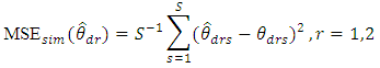 Where
Where  is the estimator for variable r in area d,
  is the s-th simulation of the estimator of variable r in area d, and
  is the true value for variable r in area d in the s-th simulation.
4.2. Results of the Simulation Experiment
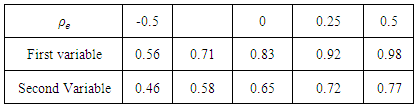
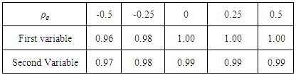
Table 1 presents the medians of the REs over the 100 areas for the different values of the correlation  with heteroscedasticity weight 1. The RE of BFH estimators are less than 1 for both variables although the gain is much better (lower value of RE) for the second variable than the first variable. The reason may be that the sampling variances are higher for the second variable than the first variable and consequently, second variable of the model borrows more strength from the first variable and hence achieves larger reduction in MSE [9]. Lowest REs are obtained for the most negative values of
  for both variables. Table 2 show the medians of the REs over D=100 areas considering heteroscedasticity weight as
  . The REs of the BFH estimators are approximately one for different values of
  for both variables. It can be said that BFH estimators performed better that UFH when homoscedastic model is considered.
 Table 1. Medians of RE over D=100 small areas with

 |
| |
|
Table 2. Medians of RE over D = 100 small areas with
 |
| |
|
5. Empirical Study
5.1. Materials and Methods
Small area models are developed using the data set of BDHS 2014 and Bangladesh Population and Housing Census 2011. The BDHS covers 600 communities (Primary Sampling Unit) across 396 sub-districts, comprising 64 districts in 7 divisions [11]. Two anthropometric standard indices Height-for-age and Weight-for-age (Z-score) are used to calculate the proportion of stunted and underweight children at district level. Three district level statistics - Proportion of children under 5 years, Proportion of household size with ≤ 4 members and Average household size are considered as explanatory variables in the FH models. The BFH model (7) as well as the UFH model (1) will be used to estimate area prevalence of the indicators. The analysis has been performed using R software.
5.2. Results of the Empirical Study
Figure 1 presents the comparison of the direct, univariate and bivariate models against sample sizes. In Bangladesh, the national level proportion of stunted and underweight children aged under 5 are estimated to be 41.0 percent and 36.0 percent respectively [11], while district level estimates obtained from SAE models vary across the districts (Panels (a) and (b)). Direct estimates are highly variable for those districts with small (≤100) sample size. However, for districts with large (>100) sample size the direct estimates are found stable and very close to the FH estimates (Panels (a) and (b)). The variation of UFH and BFH estimates are smaller than the direct estimates over the sample sizes. 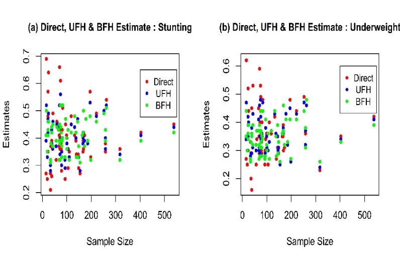 | Figure 1. Estimates of Direct, UFH and BFH Model |
 | Figure 2. Coefficient of variation of Direct, UFH and BFH estimators |
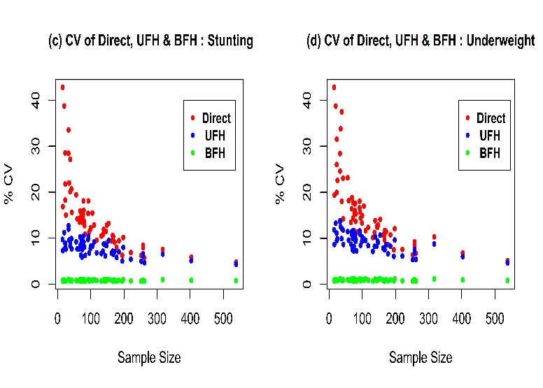
The above statements are supported by the pattern of root mean squared errors (RMSE) or coefficient of variations (CV) of the estimates. The CVs of the direct estimates are almost double those of FH estimators when the samples are small, however the differences reduce with the increasing sample size (Figure 2). For FH, CV's are found below 15 percent for all sample sizes. However, BFH estimators have lower CV’s comparing direct and UFH estimators which means BFH estimators perform better than UFH and direct estimators over the sample sizes. Figure 3 show that the direct estimates are randomly distributed around the FH estimates and they are close to the diagonal line indicating no evidence of bias. 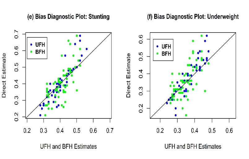 | Figure 3. Bias diagnostic plot of UFH and BFH model |
 | Figure 4. Relative Efficiencies of UFH and BFH Estimators |
 | Figure 5. Gain in efficiency of BFH over UFH estimators |
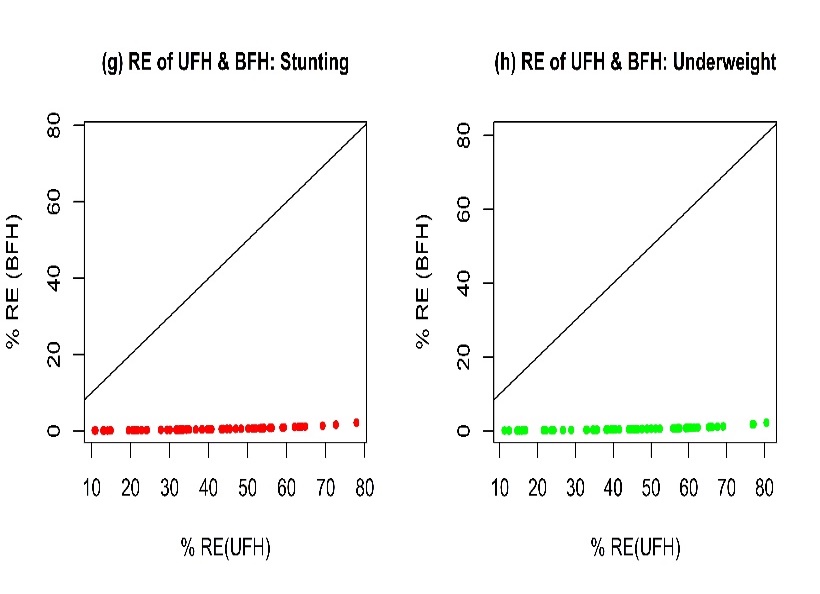
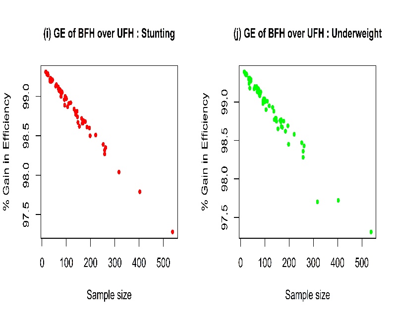
Although the differences in the UFH and BFH estimates are negligible (Figure 1), the efficiency significantly varies with sample size. Figure 4 exhibit smaller RMSE of BFH estimates than those of UFH estimates for both stunting and underweight. So from this figure it can be said that BFH estimators have quite good benefit over the UFH estimators. Figure 5 shows that the gain in efficiency (GE= ratio of difference between the RMSEs of UFH and BFH to RMSE of UFH) of BFH estimates decreases with sample size. We can say from Figure 5 that the BFH estimators perform better than UFH estimators for small sample sizes.
6. Conclusions
In conclusion, in the simulation experiment, relative efficiencies of bivariate estimators were calculated on data generated from a homoscedastic BFH model. In that case, good gains are obtained for both variables with different values of sampling errors but gains are better for the second variable. The reason is that the sampling variances were higher for the second variable than the first variable but when the data were simulated from a heteroskedastic model, resulting relative efficiencies close to 1 for both variables.BFH and UFH estimators were also applied to small area prevalences of Bangladesh Demographic Health Survey 2011 with auxiliary variables taken from the Bangladesh Population and Housing Census 2011. The study attempts to examine the small area estimates of nutritional status for Bangladeshi children under five years of age in terms of stunting and underweight. The efficiencies of BFH and UFH estimators have been compared for both variables. The distributions of the estimated coefficient of variation shows that BFH estimators had greater improvement over direct and UFH estimators for both variables. The efficiency of BFH estimates are appearing better particularly for the areas with small samples for the data set and variables considered here. These efficiencies are themselves estimates and future research will determine whether the apparent gain from the BFH are genuine with more auxiliary variables or more areas or both would be worthwhile. The research could also be extended in future incorporating multivariate version of spatio-temporal small area approach where we will consider the geographic position of the considered small areas.
References
| [1] | Rao, J. N. and Monila, I. (2015), Small Area Estimation. Hoboken, New Jersey: John Wiley and Sons. |
| [2] | Horvitz, D.G. and Thompson, D. J. (1952), A generalization of sampling without replacement from a finite universe. Journal of the American Statistical Association, 47(260), 663-685. |
| [3] | Srndal, C., Swensson, B. and Wretman, J. (1992), Model assisted Survey Sampling. New York: Springer-Verlag. |
| [4] | Chambers, R. and Clark, R. (2012), An introduction to model-based survey sampling with applications. Great Clarendon Street, Oxford: Oxford University Press. |
| [5] | Prasad, N. and Rao, J. (1990), The estimation of the mean squared error of small area estimators. Journal of the American Statistical Association, 85(409), 163-171. |
| [6] | Fay, R.E. and Herriot. R.A. (1979), Estimates of income for small places: an application of James-Stein procedures to census data. Journal of the American Statistical Association, 73(366a), 269-277. |
| [7] | Benavent, R. and Morales, D. (2016), Multivariate Fay-Herriot models for small area estimation. Computational Statistics and Data Analysis, 94, 372-390. |
| [8] | Datta. G. S., Day. B., and Maiti. T. (1998), Multivariate Bayesian Small Area Estimation: An Application to Survey and Satellite Data. Sankhya: The Indian Journal of Statistics, Series A, 60(3), 344-362. |
| [9] | Gonzalez-Manteiga, W., Lombardia, M.J., Monila, I., Morales, D. and Santamaria, L. (2008) Analytic and bootstrap approximations of prediction errors under a multivariate Fay-Herriot model. Computational Statistics and Data Analysis, 52(12), 5242-5252. |
| [10] | NIPORT, M., Associates, and International, I. (2013), Bangladesh Demographic and Health Survey 2011, Dhaka, Bangladesh, and Rockville, Maryland, U.S.A.: National Institute of Population, Research and Training (NIPORT), Mitra and Associates, and ICF International. |
| [11] | NIPORT, M., Associates, and International, I. (2016), Bangladesh Demographic and Health Survey 2011, Dhaka, Bangladesh, and Rockville, Maryland, U.S.A.: National Institute of Population, Research and Training (NIPORT), Mitra and Associates, and ICF International. |

 Abstract
 Reference
 Full-Text PDF
 Full-text HTML