-
Paper Information
- Previous Paper
- Paper Submission
-
Journal Information
- About This Journal
- Editorial Board
- Current Issue
- Archive
- Author Guidelines
- Contact Us
International Journal of Statistics and Applications
p-ISSN: 2168-5193 e-ISSN: 2168-5215
2018; 8(5): 274-290
doi:10.5923/j.statistics.20180805.06

Bayesian Survival Analysis of Topp-Leone Generalized Family with Stan
 Abstract
 Reference
 Full-Text PDF
 Full-text HTML
Mohammed H. AbuJarad, Athar Ali Khan
Department of Statistics and Operations Research, AMU, Aligarh, India
Correspondence to: Mohammed H. AbuJarad, Department of Statistics and Operations Research, AMU, Aligarh, India.
| Email: |  |
Copyright © 2018 The Author(s). Published by Scientific & Academic Publishing.
This work is licensed under the Creative Commons Attribution International License (CC BY).
http://creativecommons.org/licenses/by/4.0/

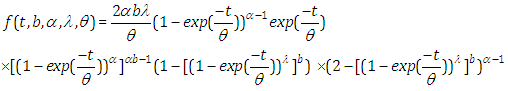
In this article, the discussion has been carried out on the generalization of three distribution by means of exponential, exponentiated exponential and exponentiated extension. We set up three and four parameters life model called the Topp-Leone exponential distribution, Topp-Leone exponentiated exponential distribution and Topp-Leone exponentiated extension distribution. We give extensive consequence of the, survival function and hazard rate function. To fit this model as survival model and hazard rate function we adopted to use Bayesian approach. A real survival data set is used to illustrate. application is done by R and Stan and suitable illustrations are prepared. R and Stan codes have been given to actualize censoring mechanism via optimization and also simulation tools.
Keywords: Topp-Leone exponential, Topp-Leone exponentiated exponential, Topp-Leone exponentiated extension, Posterior, Simulation, RStan, Bayesian Inference, R, HMC
Cite this paper: Mohammed H. AbuJarad, Athar Ali Khan, Bayesian Survival Analysis of Topp-Leone Generalized Family with Stan, International Journal of Statistics and Applications, Vol. 8 No. 5, 2018, pp. 274-290. doi: 10.5923/j.statistics.20180805.06.
Article Outline
1. Introduction
- In the survival, a number of continuous univariate distributions have been widely utilized for demonstrating information in numerous areas, for example, biology, medicine, engineering, public health, epidemiology and economics. In any case, applied areas, for example, lifetime analysis obviously require expanded types of these distributions. In this way, a few classes of distributions have been built by extending common families of continuous distributions. These generalized distributions give greater adaptability by including "at least one" parameters to the standard model. The Topp-Leone distribution was introduced by Topp and Leone in 1955 (Topp and Leone, 1955). Topp-Leone Generalized family of distributions was inferred by Rezaei et al. (2016). The distribution and density function of proposed family is known by
 | (1.1) |
 | (1.2) |
 and
and  . This present article is designed as follows; Section 2, we derive three parameter life model called Topp-Leone exponential distribution, the pdf and cdf expansion, in Section 2.1, we derive four parameter life model called Topp-Leone exponentiated exponential distribution, the pdf and cdf expansion, in Section 2.2, we derive four parameter life model called Topp-Leone exponentiated extension distribution, the pdf and cdf expansion. The fundamental properties of the proposed demonstrate including, Bayesian methodology has been received to fit this model as survival model and hazard rate function. Survival analysis is the name for an accumulation of statistical techniques used to depict and evaluate time to event data. In survival analysis we utilize the term inability to characterize the event of the interest. In this paper, an endeavor has been made to plot how Bayesian methodology continues to fit Topp-Leone exponential model, Topp-Leone exponentiated exponential and Topp-Leone exponential extension for lifetime data using Stan. The tools and techniques used in this paper are in Bayesian environment, which are implemented using rstan package. Stan is a programming language designed to make statistical modeling easier and faster, especially for Bayesian estimation problems, it can do estimate complex models with large numbers of parameters, and can generally do it faster than alternative like JAGS/BUGS. However, Simulation can also be used as an alternative technique. Simulation based on Markov chain Monte Carlo (MCMC) is used when it is not possible to sample
  directly from posterior
  . For a wide class of problems, this is the easiest method to get reliable results (Gelman et al, 2014). Gibbs sampling, Hamiltonian Monte Carlo and Metropolis-Hastings algorithm are the MCMC techniques which render difficult computational tasks quite feasible. To make computation easier, software such as R, Stan is a C++ library for Bayesian modeling and inference that primarily uses the No-U-Turn sampler (NUTS) (Hoffman and Gelman 2012) to obtain posterior simulation given specified model and data, a variant of Hamiltonian Monte Carlo (HMC) are used, Stan can produce high dimensional proposals that are accepted with high probability without having to spend time tuning. Bayesian analysis of proposal appropriation has been made with the following objectives:Ÿ To define a Bayesian model, that is, specification of likelihood and prior distribution.Ÿ To write down the R code for approximating posterior densities with, Stan.Ÿ To illustrate numeric as well as graphic summaries of the posterior densities.
2. The Topp-Leone Exponential Distribution
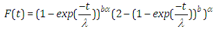
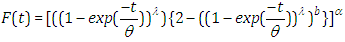
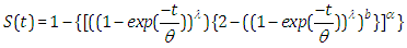
- Corderio et al. (2013) utilized the method for adding parameter prompts the exponentiated type of distribution which was considered by Nadarajah and Kotz (2003). In this segment, we infer three parameter Topp-Leone Exponential distribution. To construct the probability density function (pdf) and cumulative distribution function (cdf) of Exponential distribution which are given by (2.3) and (2.4), individually,
 | (2.3) |
 | (2.4) |
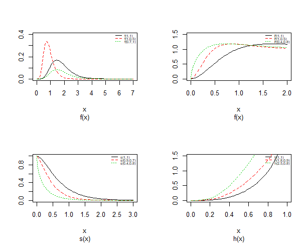
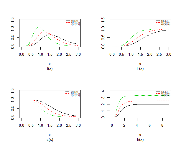 | Figure 1. Probability density plots, cdf, survival and hazard curves of Topp-Leone Exponential distribution for different value |
 | (2.5) |
 | (2.6) |
 | (2.7) |
 | (2.8) |
2.1. The Topp-Leone Exponentiated Exponential Distribution
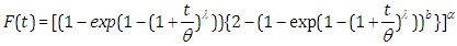
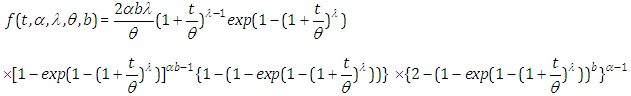
- Topp-Leone additional two shapes parameter to the two-parameter exponentiated exponential distribution. It is seen that the new four-parameter distribution is exceptionally adaptable. At the point when the pdf, cdf, survival function and hazard function of exponentiated exponential appropriation is
 , the outcomes are (2.9), (2.10), (2.11) and (2.12), individually, as in Figure(2)
 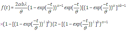 | (2.9) |
 | (2.10) |
 | (2.11) |
 | (2.12) |
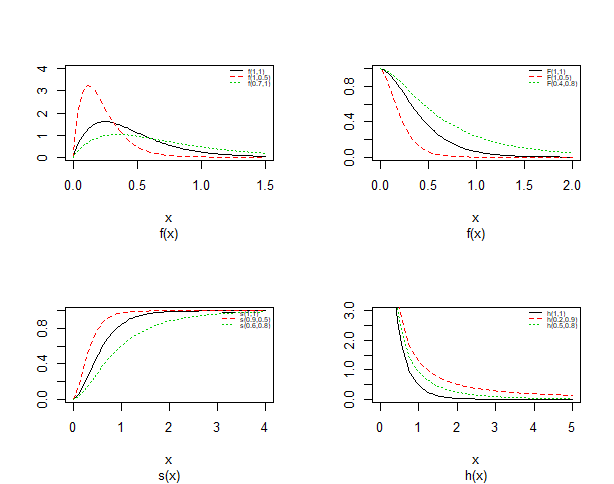
 | Figure 2. Probability density plots, cdf, survival and hazard curves of Topp-Leone Exponential distribution for different value |
2.2. The Topp-Leone Exponential Extension Distribution
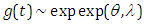
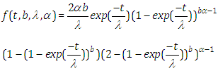
- When the pdf, cdf, survival function and hazard function of exponential extension distribution is
 , the results are (2.13), (2.14), (2.15) and (2.16), respectively, as in Figure(3)
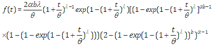 | (2.13) |
 | (2.14) |
 | (2.15) |
 | (2.16) |
 | Figure 3. Probability density plots, cdf, survival and hazard curves of Topp-Leone Exponential distribution for different value |
3. Bayesian Inference
- Gelman et al., (2013) break applied Bayesian modeling into the following three steps:1. Set up a full probability model for all observable and unobservable quantities. This model should be consistent with existing knowledge of the data being modeled and how it was collected.2. Calculate the posterior probability of unknown quantities conditioned on observed quantities. The unknowns may include unobservable quantities such as parameters and potentially observable quantities such as predictions for future observations.3. Evaluate the model fit to the data. This includes evaluating the implications of the posterior.Typically, this cycle will be repeated until a sufficient fit is achieved in the third step. Stan automates the calculations involved in the second and third steps (Carpenter et al., 2017).We have to specify here the most vital in Bayesian inference which are as per the following:Ÿ prior distribution:
 The parameter
  can set a prior distribution elements that using probability as a means of quantifying uncertainty about
  before taking the data into acount.Ÿ Likelihood
  likelihood function for variables are related in full probability model.Ÿ Posterior distribution
  is the joint posterior distribution that expresses uncertainty about parameter
  after considering about the prior and the data, as in equation.
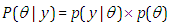 | (3.17) |
4. The Prior Distributions
- The Bayesian inference, having the prior distribution, can provide the information concerning an uncertain parameter
 connected through the probability distribution of data. This uncertain parameter is able to help obtain the posterior distribution
  . In the case of the Bayesian paradigm, it is very important for prior information to be identified through the value of the specified parameter. The information which are gathered before analyzing the experimental data with using a probability distribution function is referred to as the prior probability distribution (or the prior). In the remain of this paper, The researchers make use of two types of priors: half-Cauchy prior and Normal prior. The simplest types of priors is a conjugate prior which facilitates posterior calculations. In addition, a conjugate prior distribution is intended for an unknown parameter which leads to a posterior distribution for which there is a simple formula for posterior means and variances. (Akhtar and Khan, 2014a) apply the half-Cauchy distribution by scale parameter
  while a prior distribution for scale parameter.Hereinafter we determination talk about the types of prior distribution: • Half-Cauchy prior. • Normal prior.First, the probability density function of half-Cauchy distribution by scale parameter
  is specified as a result
 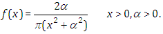 Half-Cauchy distribution does not exist for mean and variance, although its mode is equal to 0. The half-Cauchy distribution by scale
  is a suggested, default, weakly informative prior distribution used for a scale parameter. On this scale
  , the density of half-Cauchy is almost flat however not completely (see Figure 4), prior distributions that are not completely flat afford adequate information for the numerical approximation algorithm to continue to look at the target density; the posterior distribution. The inverse-gamma is often used as a non-informative prior distribution for scale parameter, but; this model creates a trouble for scale parameters close to zero; (Gelman and Hill, 2007) suggest that, the uniform, otherwise if more information is needed, the half-Cauchy is a better option. Consequently, in this paper, the half-Cauchy distribution with scale parameter
  is used as a weakly informative prior distribution.
 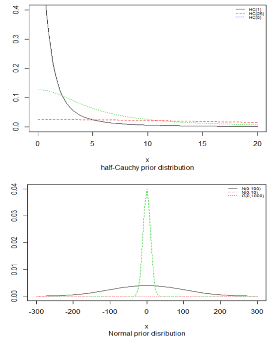 | Figure 4 |
 independently in the normal distribution with mean=0 and standard deviation=1000, i.e.,
 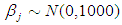 , for this, we get a flat prior. As of (Figure 4), we see that the large variance indicates a lot of uncertainty about each parameter and hence, a weak informative distribution.
 5. Stan Modeling
- Stan is an abnormal state dialect written in a C++ library for Bayesian demonstrating and (Carpenter et al., 2017) is another Bayesian programming program for induction that essentially utilizes the No-U-Turn sampler (NUTS) (Hoffman and Gelman 2012) to get posterior simulations given a client indicated model and data. Hamiltonian Monte Carlo (HMC; Radford 2011; Betancourt 2017) is one of the calculations having a place with the general class of MCMC strategies. Practically speaking, HMC can be very complex, because in addition to the specific computation of possibly complex derivatives, it requires tweaking of a few parameters. Hamiltonian Monte Carlo requires a touch of exertion to program and tune. In more entangled settings, however, HMC to be quicker and more dependable than fundamental Markov chain reproduction, Gibbs sampler and the Metropolis algorithm because they explores the posterior parameter space more efficiently. they do so by pairing each model parameter with a momentum variable, which determines HMC exploration behavior of the target distribution based on the posterior density of the current drawn parameter and hence enable HMC to suppress the random walk behavior in the Metropolis algorithm (Gelman, Carlin, Stern, & Rubin, 2014, p. 300). Consequently, Stan is considerably more efficient than the traditional Bayesian software programs. However, the main function in the rstan package is Stan, which calls the Stan software program to estimate a specified statistical model, rstan provides a very clever system in which most of the adaptation is automatic. Statistical model through a conditional probability function
 can be classified by Stan program, where
  is a sequence of modeled unknown values,
  is a sequence of modeled known values, and
  is a sequence of un-modeled predictors and constants (e.g., sizes, hyperparameters). A Stan program imperatively defines a log probability function over parameters conditioned on specified data and constants. Stan provides full Bayesian inference for continuous-variable models through Markov chain Monte Carlo methods (Metropolis et al., 1953), an adjusted form of Hamiltonian Monte Carlo sampling (Duane et al., 1987; Neal, 1994). Stan can be called from R using the rstan package, and through Python using the pystan package. All interfaces support sampling and optimization-based inference with diagnostics and posterior analysis. rstan and pystan also provide access to log probabilities, parameter transforms, and specialized plotting. Stan programs consist of variable type declarations and statements. Variable types include constrained and unconstrained integer, scalar, vector, and matrix types. Variables are declared in blocks corresponding to the variable use: data, transformed data, parameter, transformed parameter, or generated quantities.
6. Bayesian Analysis of Model
- Bayesian analysis is the strategy to acquire the marginal posterior distribution of the specific parameters of interest. On a fundamental level, the course to accomplishing this point is clear; first, we require the joint posterior distribution of every obscure parameter, at that point, we integrate this distribution over the unknowns parameters that are not of prompt enthusiasm to acquire the coveted marginal distribution. Or on the other hand identically, utilizing simulation, we draw samples from the joint posterior distribution, at that point, we take at the parameters of interest and disregard the estimations of the other obscure parameters.
6.1. Topp-Leone Exponential Model
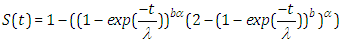
- Presently, the probability density function (pdf) is given by
 Likewise, the survival function is given by
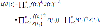
 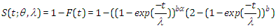 We can express the likelihood function for right censored (similar to our case the data are right censored) as
 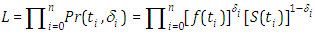 where
where  is a pointer variable which takes esteem 0 if perception is censored and 1 if perception is uncensored. In this manner, the likelihood function is given by
 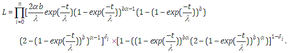 | (6.18) |
 | (6.19) |
 and
and  . We talked about the issue related with determining prior distributions in section 4, however, for effortlessness now, we expect that the prior distribution for
  and
and  is half-Cauchy on the interval [0, 5] and for
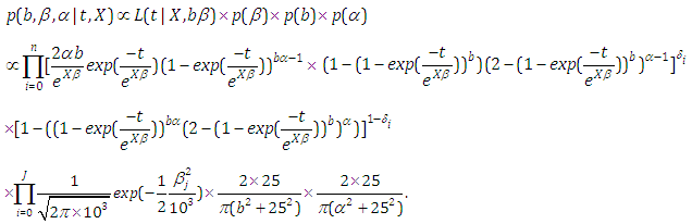
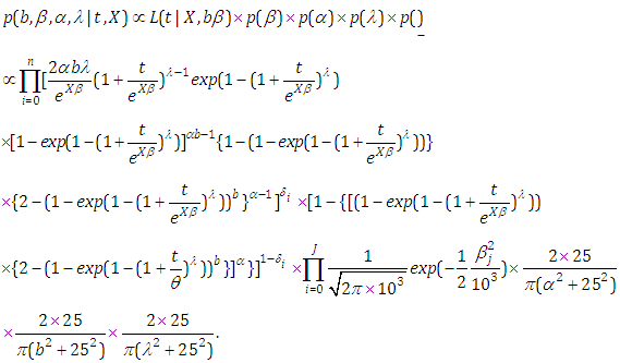
  is Normal with [0, 5]. Rudimentary utilization of Bayes control as showed in (3.17), connected to (6.18), at that point gives the posterior density for
  and
and  as equation (6.19). Result for this marginal posterior distribution get high-dimensional integral over every single model parameters
  and
and  . To unravel this integral, we utilize the approximated utilizing Markov Chain Monte Carlo methods techniques. be that as it may, because of the accessibility of computer software package like rstan, this required model can without much of a stretch be fitted in Bayesian paradigm utilizing Stan in addition to MCMC strategies.
6.2. Topp-Leone Exponentiated Exponential Model
- Now, the probability density function (pdf) is given by
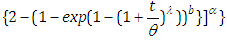
 Also, the survival function is given by
  In the presence of censoring, the resulting log-likelihood function is modified to account for the possibility of partially observed data (in correspondence with censoring) We can write the likelihood function for right censored (as is our case the data are right censored) as
 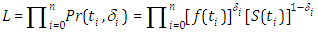 where
where  is an indicator variable which takes value 0 if observation is censored and 1 if observation is uncensored. Thus, the likelihood function is given by
 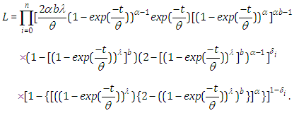 | (6.20) |
 | (6.21) |
 and
and  We discussed the issue associated with specifying prior distributions in section 4, but for simplicity at this point, we assume that the prior distribution for
  ,
,  and
and  is half-Cauchy on the interval [0, 5] and for
  is Normal with [0, 5]. Elementary application of Bayes rule as displayed in (3.17), applied to (6.20), then gives the posterior density for
  and
and  as equation (6.21). The result for this marginal posterior distribution get high-dimensional integral over all model parameters
  and
and  . To resolve this integral we use the approximated using Markov chain Monte Carlo methods. However, due to the availability of computer software package like rstan, this required model can easily fit in Bayesian paradigm using Stan as well as MCMC techniques.
6.3. Topp-Leone Exponential Extension Model
- The probability density function (pdf) given by
 The survival function is given by
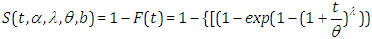
 We can state the likelihood function for right censored (as is our case the data are right censored) as
 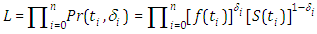 where
where  is an indicator variable which takes value if observation is censored and 1 if observation is uncensored. Thus, the likelihood function is given by
 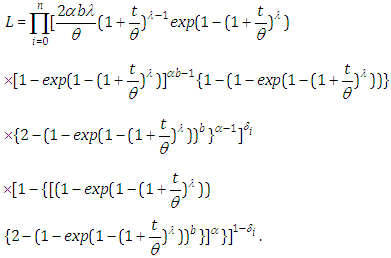 | (6.22) |
 | (6.23) |
 and
and  . We discussed the issue associated with specifying prior distributions in section 4, but for simplicity at this point, we assume that the prior distribution for
  and
and  is half-Cauchy on the interval [0, 5] and for
  is Normal with [0, 5]. Elementary application of Bayes rule as displayed in (3.17), applied to (6.22), then gives the posterior density for
  and
and  as equation (6.23). The result for this marginal posterior distribution get high-dimensional integral over all model parameters
  and
and  . To resolve this integral we use the approximated using Markov chain Monte Carlo methods. However, due to the availability of computer software package like rstan, this required model can easily fit in Bayesian paradigm using Stan as well as MCMC techniques.
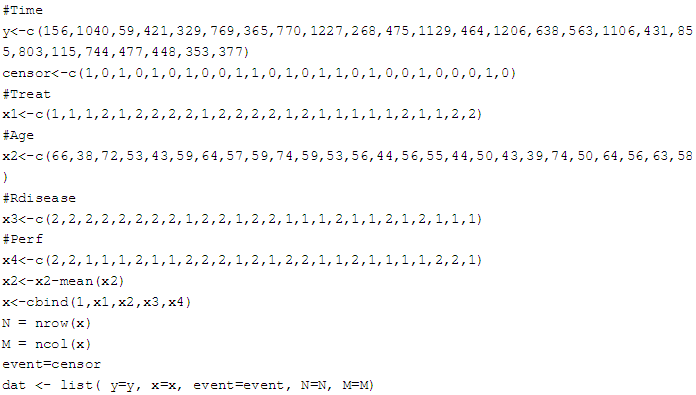
6.4. The Data: Chemotherapy in Ovarian Cancer Patients
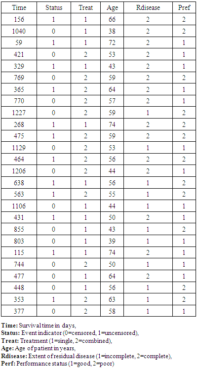
- Following careful treatment od ovarian malignancy, patients may experience a course of chemotherapy. The two distinct types of chemotherapy treatment, Edmunson et al. (1979) looked at the counter tumor impacts of cyclophosphamide alone and cyclophosphamide joined with adriamycin. The preliminary included 26 ladies with insignificant remaining illness and who had encountered careful extraction of all tumor masses more prominent that 2 can in dimeter. Following surgery, the patients were additionally ordered by whether the lingering illness was totally or mostly extracted. The age of the patient and their execution status were likewise recorded toward the beginning of the preliminary. The reaction variable was the survival time in day following randomisation to one ar other of the two chemotherapy medications. The data, which were obtained from Therneau (1986), are given in Table (1):
|
7. Implementation Using Stan
- Bayesian modeling of Topp-Leone models in rstan package includes the creation of blocks, data, transformed data, parameter, transformed parameter, or generated quantities. To use the method for Topp-Leone exponential model, Topp-Leone exponentiated exponential, and Topp-Leone exponential extension, we will follow the following steps; starting with build a function for the model containing the accompanying items:Ÿ Define the log survival.Ÿ Define the log hazard.Ÿ Define the sampling distributions for right censored data.At that point the distribution ought to be built on the function definition blocks. The function definition block contains user defined functions. The data block states the needed data for the model. The transformed data block permits the definition of constants and transforms of the data. The parameters block declares the model parameters. The transformed parameters block allows variables to be defined in terms of data and parameters that may be used later and will be saved. The model block is where the log probability function is defined.
7.1. Model Specification
- Presently we will look at the posterior estimates of the parameters when the Topp-Leone exponential, Topp-Leone exponentiated exponential and Topp-Leone exponential expansion model’s are fitted to the previously mentioned data (information). Accordingly the importance of the likelihood (probability) turns into the highest need for the Bayesian fitting. Indicate statistical models utilizing the Stan modeling language, which is detailed in the manual of Stan (The Stan Development Team 2014c). Here, we have likelihood as:
 along these lines, our log-likelihood progresses toward getting to be
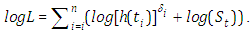
7.1.1. Topp-Leone Exponential Model
- The first model is Topp-Leone exponential:
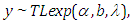 where
where  a linear combination of explanatory variables, log is the natural log for the time to failure event. The Bayesian system requires the determination and specification of prior distributions for the parameters. Here, we stick to subjectivity and thus introduce weakly informative priors for the parameters. Priors for the
  and
and  are taken to be half-Cauchy and normal as follows:
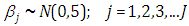
 The rstan package allows a model to be coded in a text file, here we write the Stan model code and save it in a separated text-file with name "model code1":
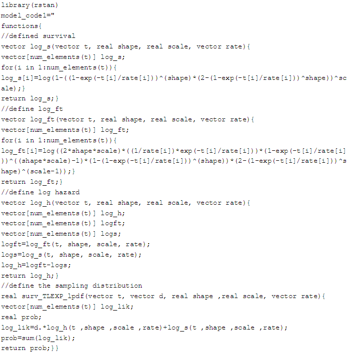 In this manner, we acquire the survival and hazard of the Topp-Leone Exponential model.
 7.1.2. Topp-Leone Exponentiated Exponential Model
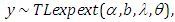
- The second model is Topp-Leone exponentiated exponential model:
 where
where  . The Bayesian framework requires the specification of prior distributions for the parameters. Here, we stick to subjectivity and thus introduce weakly informative priors for the parameters. Priors for the
 and
and  are taken to be normal and half-Cauchy as follows:
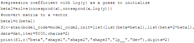
 To fit this model in Stan, we first write the Stan model code and save it in a separated text-file with name "model code2".:
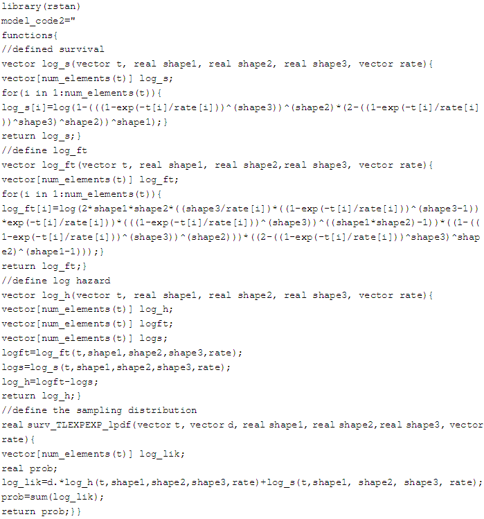 Therefore, we obtain the survival and hazard of the Topp-Leone exponentiated exponential model.
7.1.3. Topp-Leone Exponential Extension Model
- The third model is Topp-Leone exponential extension model:
 where
where  The Bayesian framework requires the specification of prior distributions for the parameters. Here, we stick to subjectivity and thus introduce weakly informative priors for the parameters. Priors for the
 and
and  are taken to be normal and half-Cauchy as follows:
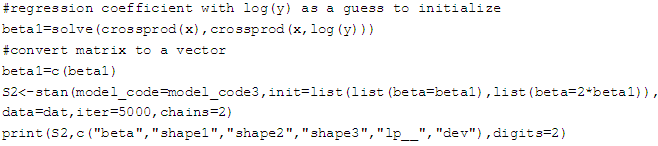
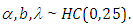 To fit this model in Stan, we first write the Stan model code and save it in a separated text-file with name "model code3":
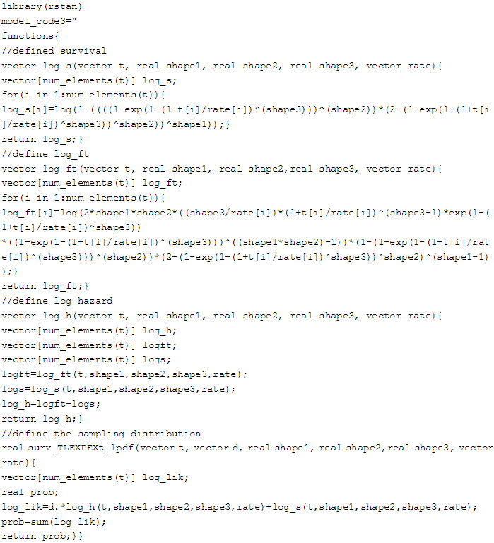 Therefore, we obtain the survival and hazard of the Topp-Leone exponential extension model.
 7.2. Build the Stan
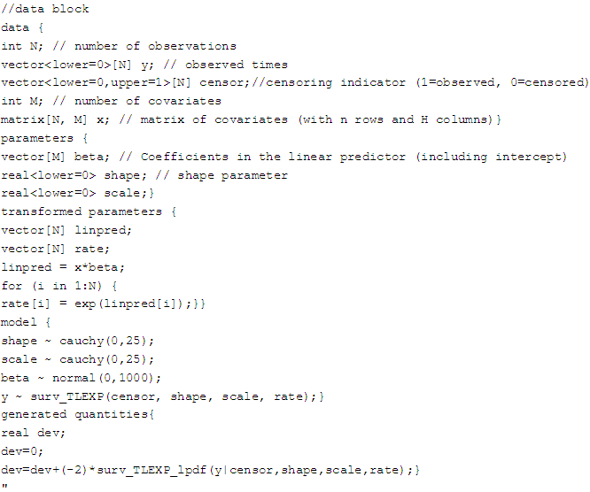
- Stan contains an arrangement of blocks as stated previously; in the first block we will define the data block, in which we include the number of the observations, observed times, censoring indicator (1=observed, 0=censored), number of covariates, and build the matrix of covariates (with N rows and M columns). Then we create the parameter in block parameters, since we have more one parameter, we will do some changes for the parameters in side transformed parameters block. Finally, we arrange the model in blocks model. In these blocks, we put the prior for the parameters and the likelihood to get the posterior distribution for these model. We save this work in a file to use it in rstan package.
7.2.1. Topp-Leone Exponential Model
7.2.2. Topp-Leone Exponentiated Exponential Model

7.2.3. Topp-Leone Exponential Extension Model
7.3. Creation of Data for Stan
- Within this part, we force organize the data that we have to utilize for analysis, data arrangement requires model matrix X, number of predictors M, information regarding censoring and response variable. The number of observations is specified by N, that is, 26. Censoring is taken into account, where 0 stands for censored and 1 for uncensored values. Finally, every one of these things are consolidated in a recorded list as dat.
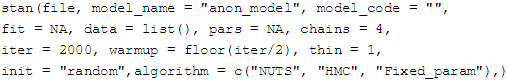
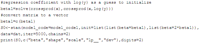
7.4. Runing the Model Using Stan for Topp-Leone Exponential Model
- Now we run Stan with 2 chains for 5000 iterations and display the results numerically and graphically:
7.4.1. Summarizing Output
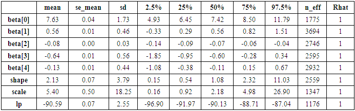
- A summary of the parameter distributions can be obtained by using print(S0), which provides posterior estimates for each of the parameters in the model. Before any inferences can be made, however, it is critically important to determine whether the sampling process has converged to the posterior distribution. Convergence can be diagnosed in several different ways. One way is to look at convergence statistics such as the potential scale reduction factor, Rhat (Gelman & Rubin, 1992), and the effective number of samples, n_eff (Gelman et al., 2013), both of which are outputs in the summary statistics with print(S0). The function rstan approximates the posterior density of the fitted model and posterior summaries can be seen in the following tables. Table 2, which contain summaries for all chains merged and individual chains, respectively. Included in the summaries are (quantiles), (means), standard deviations (sd), effective sample sizes (n_eff), and split (Rhats) (the potential scale reduction derived from all chains after splitting each chain in half and treating the halves as chains). For the summary of all chains merged, Monte Carlo standard errors (se_mean) are also reported.
 is
is  and 95% credible interval is
  , which is statistically significant. Rhat is close to 1.0, indication of good mixing of the three chains and thus approximate convergence. posterior estimate for
  is
is  and 95% credible interval is
  , which is statistically not significant. Rhat is close to 1.0, indication of good mixing of the three chains and thus approximate convergence posterior estimate for
  is
is  and 95% credible interval is
 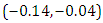 , which is statistically significant. Rhat is close to , indication of good mixing of the three chains and thus approximate convergence, posterior estimate for
  is
is  and 95% credible interval is
  , which is statistically not significant. Rhat is close to , indication of good mixing of the three chains and thus approximate convergence, posterior estimate for
  is
is  and 95% credible interval is
  , which is statistically not significant. Rhat is close to , indication of good mixing of the three chains and thus approximate convergence. The table displays the output from Stan. Here, the coefficient
  is the intercept, while the coefficient
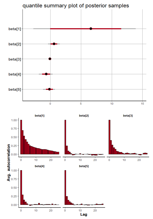
  is the effect of the covariate included in the model. The effective sample size given an indication of the underlying autocorrelation in the MCMC samples values close to the total number of iterations. The selection of appropriate regressor variables can also be done by using a caterpillar plot. Caterpillar plots are popular plots in Bayesian inference for summarizing the quantiles of posterior samples. we can see in this (Figure 5) that the caterpillar plot is a horizontal plot of 3 quantiles of selected distribution, in this plot, credible intervals (by default 80%) for all the parameters, and the median of each chain are displayed. In addition, under the lines representing intervals, small colored areas are used to indicate which range the value of the split
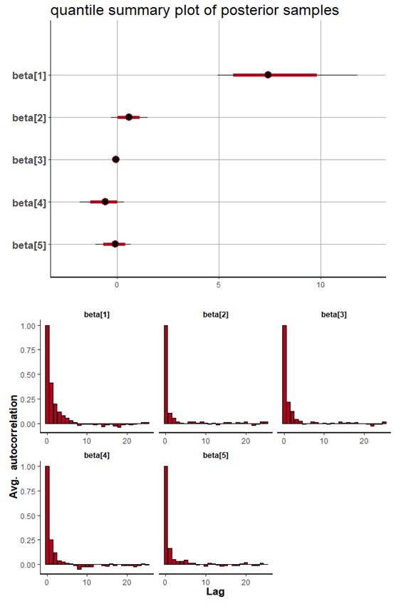
  statistic is in. This may be used to produce a caterpillar plot of posterior samples. In MCMC estimation, it is important to thoroughly assess convergence as it in (Figure 6) the rstan contains specialized function to visualise the model output and assess convergence.
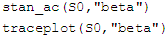
 | Figure 5. Caterpillar plot for Topp-Leone Exponential model |
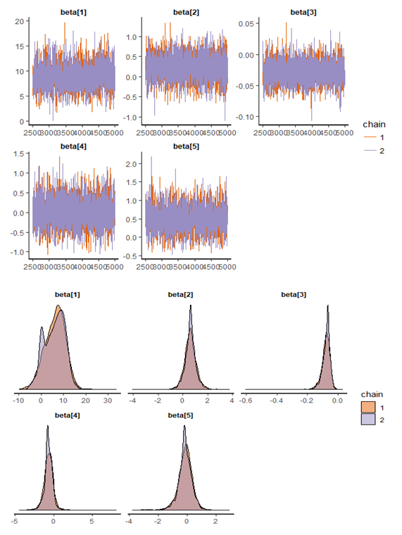
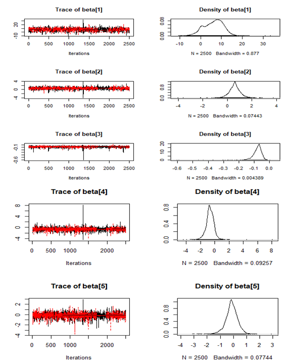
 | Figure 6. Checking model convergence using rstan, through inspection of the traceplots or the autocorrelation plot |
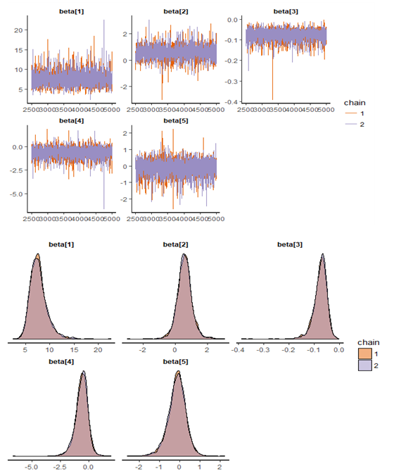
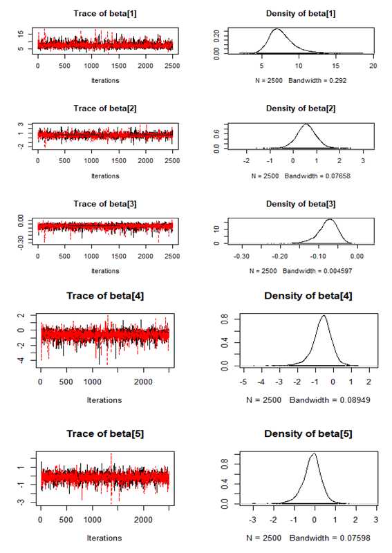 | Figure 7. Checking model convergence using coda, through inspection of the simulated posterior density plots with trace plots of regressor variables obtained by HMC |
7.5. Runing the Model Using Stan for Topp-Leone Exponentiated Exponential Model
- Now we run Stan with 2 chains for 5000 iterations and display the results numerically and graphically:
7.5.1. Summarizing Output
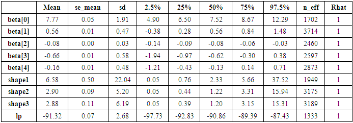
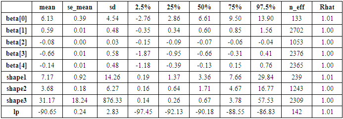
- The function rstan approximates the posterior density of the fitted model and posterior summaries can be seen in the following tables. Table 2, contains summaries for for all chains merged and individual chains, respectively. Included in the summaries are (quantiles), (means), standard deviations (sd), effective sample sizes (n_eff), and split (Rhats) (the potential scale reduction is derived from all chains after splitting each chain in half and treating the halves as chains). For the summary of all chains merged, Monte Carlo standard errors (se_mean) are also reported. The inference of the posterior density after fitting the (Topp-Leone exponential exponential model) for ovarian cancer patients data using stan are reposted in Table 3. The posterior estimate for
 is
is  and 95% credible interval is
  , which is statistically significant. Rhat is close to
  , indication of good mixing of the three chains and thus approximate convergence. posterior estimate for
  is
is  and 95% credible interval is
  , which is statistically not significant. Rhat is close to
  , indication of good mixing of the three chains and thus approximate convergence posterior estimate for
  is
is  and 95% credible interval is
  , which is statistically significant. Rhat is close to
  , indication of good mixing of the three chains and thus approximate convergence, posterior estimate for
  is
is  and 95% credible interval is
  , which is statistically not significant. Rhat is close to
  , indication of good mixing of the three chains and thus approximate convergence, posterior estimate for
  is
is  and 95% credible interval is
  , which is statistically not significant. Rhat is close to
  , indication of good mixing of the three chains and thus approximate convergence. The selection of appropriate regressor variable can also be done by using a caterpillar plot. Caterpillar plots are popular plots in Bayesian inference for summarizing the quantiles of posterior samples. we can see in this (Figure 8) that the caterpillar plot is a horizontal plot of 3 quantiles of selected distribution. In MCMC estimation, it is important to thoroughly assess convergence as in (Figure 9) the rstan contains specialized function to visualise the model output and assess convergence.
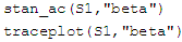
|
 | Figure 8. Caterpillar plot for Topp-Leone Exponentiated Exponential model |
 | Figure 9. Checking model convergence using rstan, through inspection of the traceplots or the autocorrelation plot |
 | Figure 10. Checking model convergence using coda, through inspection of the simulated posterior density plots with trace plots of regressor variables obtained by HMC |
7.6. Runing the Model Using Stan for Topp-Leone Exponential Extension Model
- Now we run Stan with 2 chains for 5000 iterations and display the results numerically and graphically:
7.6.1. Summarizing Output
- The function rstan approximates the posterior density of the fitted model, and posterior summaries can be seen in the following tables. Table 4, contains summaries for for all chains merged and individual chains, respectively. Included in the summaries are (quantiles),(means), standard deviations (sd), effective sample sizes (n_eff), and split (Rhats) (the potential scale reduction derived from all chains after splitting each chain in half and treating the halves as chains). For the summary of all chains merged, Monte Carlo standard errors (se_mean) are also reported. The inference of the posterior density after fitting the (Topp-Leone exponential extension model) for ovarian cancer patients data using stan are reposted in Table 4. The posterior estimate for
 is
is  and 95% credible interval is
  , which is statistically not significant. Rhat is close to 1.0, indication of good mixing of the three chains and thus approximate convergence. posterior estimate for
  is
is  and 95% credible interval is
  , which is statistically not significant. Rhat is close to
  , indication of good mixing of the three chains and thus approximate convergence posterior estimate for
  is
is  and 95% credible interval is
  , which is statistically significant. Rhat is close to
  , indication of good mixing of the three chains and thus approximate convergence, posterior estimate for
  is
is  and 95% credible interval is
  , which is statistically not significant. Rhat is close to 1.0, indication of good mixing of the three chains and thus approximate convergence, posterior estimate for
  is
is  and 95% credible interval is
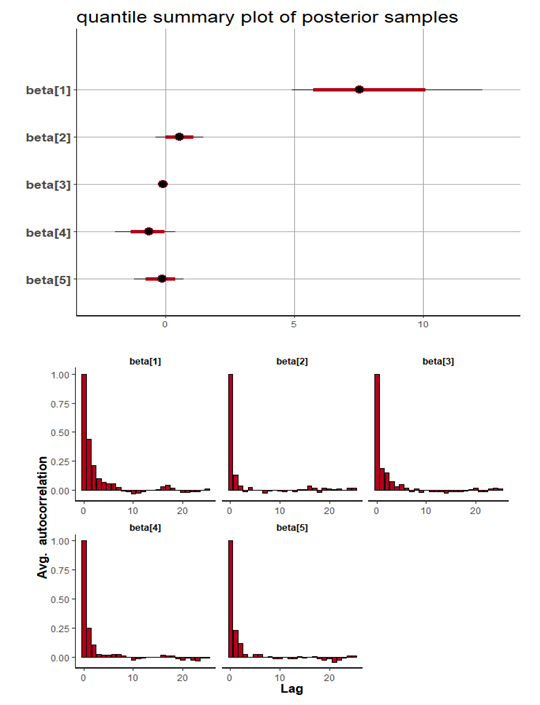
  , which is statistically not significant. Rhat is close to 1.0, indication of good mixing of the three chains and thus approximate convergence. The selection of appropriate regressor variable can also be done by using a caterpillar plot. Caterpillar plots are popular plots in Bayesian inference for summarizing the quantiles of posterior samples. We can see in (Figure 11) that the caterpillar plot is a horizontal plot of 3 quantiles of selected distribution. In MCMC estimation, it is important to thoroughly assess convergence as it in (Figure 12) the rstan contains specialized function to visualise the model output and assess convergence
|
 | Figure 11. Caterpillar plot for Topp-Leone Exponential Extension model |
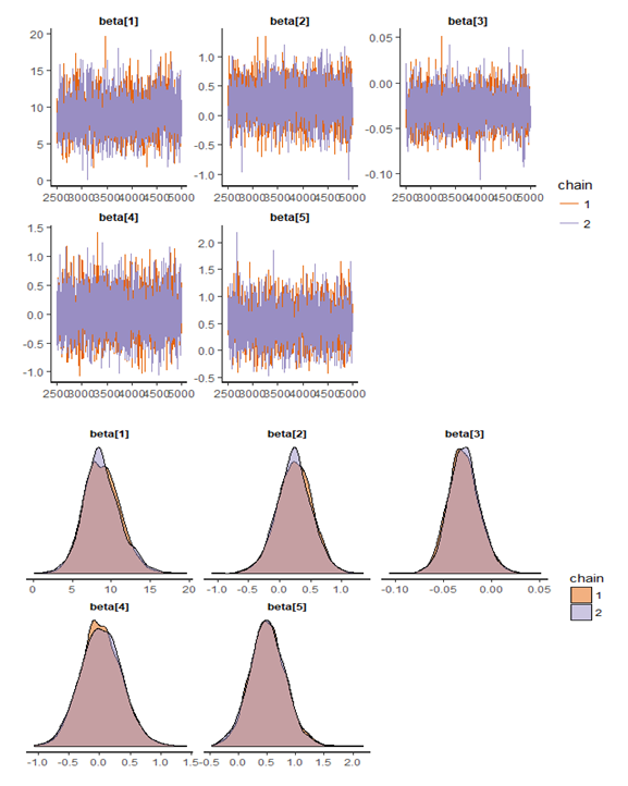
 | Figure 12. Checking model convergence using rstan, through inspection of the traceplots or the autocorrelation plot |
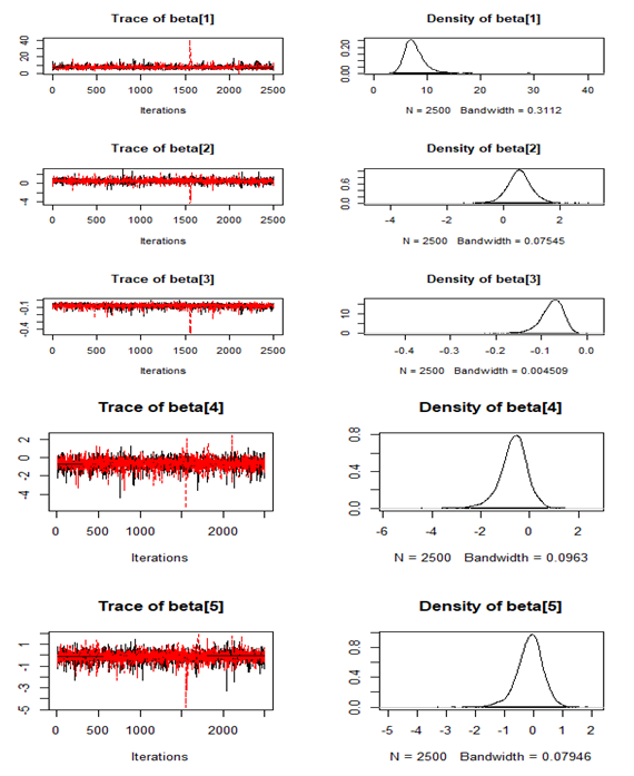
 | Figure 13. Checking model convergence using coda, through inspection of the simulated posterior density plots with trace plots of regressor variables obtained by HMC |
8. Conclusions
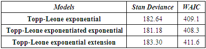
- It is a standout amongst the most critical issues in Bayes statistics how to make accurate Markov Chain Monte Carlo (MCMC) process. Here there are some MCMC methods, for example, the Metropolis method, the Gibbs sampler method, and Hamiltonian Monte Carlo method (HMC). Another problems is how we know which model best. Numerical calculation of widely applicable information criterion (WAIC, Watanabe 2010) and deviance, are help a lot for this tow problems depends on the accuracy of MCMC process and models. Here, therefore, Table 5 clearly demonstrates that Topp-Leone exponentiated exponential is the most proper model for the Stan as it has least estimation of deviance and WAIC, when contrasted with Topp-Leone exponential and Topp-Leone exponential extension.
|
References
| [1] | Akhtar, M. T. and Khan, A. A. (2014a). Bayesian analysis of generalized log-Burr family with R. Springer Plus, 3-185. |
| [2] | Carpenter, B., Gelman, A., Hoffman, M., Lee, D., Goodrich, B., Betancourt, M., & . Riddell, A. (2017). Stan: A probabilistic programming language. Journal of Statistical Software, 76, 1-32. |
| [3] | Cordeiro, G. M., Ortega, E. M. and da Cunha, D. C. C. (2013). The exponentiated generalized class of distributions. Journal of Data Science, 11, 1-27. |
| [4] | Duane, A., Kennedy, A., Pendleton, B., and Roweth, D. (1987). Hybrid Monte Carlo. Physics Letters B, 195(2): 216-222. 24. |
| [5] | Edmunson, J.H., Fleming, T.R., Decker, D.G., Malkasian, G.D., Jorgenson, E.O., Jeffries, J.A., Webb, M.J. and Kvols, L.K. (1979). Different chemotherapeutic sensitivities and host factors affecting prognosis in advanced ovarian carcinoma versus minimal residual disease. Cancer Treatment Reports, 63, 241-7. |
| [6] | Gelman, A., Carlin, J. B., Stern, H. S., and Rubin, D. B. (2014). Bayesian Data Analysis (3rd ed.), Chapman and Hall/CRC, New York. |
| [7] | Gelman, A., Carlin, J. B., Stern, H. S., Dunson, D. B., Vehtari, A., and Rubin, D. B. (2013). Bayesian Data Analysis. Chapman &Hall/CRC Press, London, third edition. |
| [8] | Gelman, A. and Hill, J. (2007) Data Analysis Using Regression and Multilevel/Hierarchical Models. Cambridge University Press, New York. |
| [9] | Hoffman, Matthew D., and Andrew Gelman. (2012). "The No-U-Turn Sampler: Adaptively Setting Path Lengths in Hamiltonian Monte Carlo." Journal of Machine Learning Research. |
| [10] | Metropolis, N., Rosenbluth, A., Rosenbluth, M., Teller, M., and Teller, E. (1953). Equations of state calculations by fast computing machines. Journal of Chemical Physics, 21: 1087-1092. 24, 25, 354. |
| [11] | Mohammed H AbuJarad and Athar Ali Khan. 2018, Exponential Model: A Bayesian Study with Stan. Int J Recent Sci Res. 9(8), pp. 28495-28506. DOI: http://dx.doi.org/10.24327/ijrsr.2018.0908.2470. |
| [12] | Nadarajah, S. and Kotz, S. (2003). Moments of some J-shaped distributions. Journal of Applied Statistics, 30, 311-317. |
| [13] | Rezaei, S., Sadr, B. B., Alizadeh, M., and Nadarajah, S. (2016). Topp-Leone Geneated Family of distribution: Properties and applications. Communications in Statistics-Theory and Methods, 46(6): 2893-2909. |
| [14] | Sangsanit, Y. and Bodhisuwan, W. (2016). The topp-leone generator of distributions: properties and inferences. Songklanakarin Journal of Science & Technology, 38(5). |
| [15] | Statisticat LLC (2015). Laplaces Demon: Complete Environment for Bayesian Inference. R package version 3.4.0, http://www.bayesian-inference.com/software. |
| [16] | Neal, R. M. (1994). An improved acceptance procedure for the hybrid monte carlo algorithm. Journal of Computational Physics, 111:194-203. 24. |
| [17] | Therneau, T.M. (1986). The COXREGR Procedure. In SAS SUGI Supplemental Library User’s Guide, version 5 edn, SAS Institute Inc., Cary, North Carolina. |
| [18] | Topp, C. W. and Leone, F. C. (1955). A family of j-shaped frequency function. Journal of the American Statistical Association, 50(269): 209-219. |