1. Introduction

Multicollinearity is a condition that arises in multiple regression analysis when there is a strong correlation or relationship between two or more explanatory variables. Multicollinearity can create inaccurate estimates of the regression coefficients, inflate the standard errors of the regression coefficients, deflate the partial t-tests for the regression coefficients, give false, nonsignificant, p-values, and degrade the predictability of the model [1, 2]. Since multicollinearity is a serious problem when we need to make inferences or looking for predictive models, it is very important to find a best suitable method to deal with multicollinearity [3].

There are several methods of detecting multicollinearity. Some of the common methods are by using pairwise scatter plots of the explanatory variables, looking at near-perfect relationships, examining the correlation matrix for high correlations and the variance inflation factors (VIF), using eigenvalues of the correlation matrix of the explanatory variables and checking the signs of the regression coefficients [4, 5].

Several solutions for handling multicollinearity problem have been developed depending on the sources of multicollinearity. If the multicollinearity has been created by the data collection, collect additional data over a wider X-subspace. If the choice of the linear model has increased the multicollinearity, simplify the model by using variable selection techniques. If an observation or two has induced the multicollinearity, remove those observations. When these steps are not possible, one might try ridge regression (RR) as an alternative procedure to the OLS method in regression analysis which suggested by [6].

Ridge Regression is a technique for analyzing multiple regression data that suffer from multicollinearity. By adding a degree of bias to the regression estimates, RR reduces the standard errors and obtains more accurate regression coefficients estimation than the OLS. Other techniques, such as LASSO and principal components regression (PCR), are also very common to overcome the multicollinearity. This study will explore LASSO, RR and PCR regression which performs best as a method for handling multicollinearity problem in multiple regression analysis.

2. Parameter Estimation in Multiple Regression

2.1. Ordinary Least Squares (OLS)

The multiple linear regression model and its estimation using OLS method allows to estimate the relation between a dependent variable and a set of explanatory variables. If data consists of n observations and each observation i includes a scalar response y_i and a vector of p explanatory (regressors) x_ij for j=1,...,p, a multiple linear regression model can be written as where is the vector dependent variable, represents the explanatory variables, is the regression coefficients to be estimated, and represents the errors or residuals. 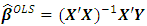is estimated regression coefficients using OLS by minimizing the squared distances between the observed and the predicted dependent variable [1, 4]. To have unbiased OLS estimation in the model, some assumptions should be satisfied. Those assumptions are that the errors have an expected value of zero, that the explanatory variables are non-random, that the explanatory variables are lineary independent, that the disturbance are homoscedastic and not autocorrelated. Explanatory variables subject to multicollinearity produces imprecise estimate of regression coefficients in a multiple regression. There are some regularized methods to deal with such problems, some of them are RR, LASSO and PCR. Many studies on the three methods have been done for decades, however, investigation on RR, LASSO and PCR is still an interesting topic and attract some authors until recent years, see e.g. [7-12] for recent studies on the three methods.

2.2. Regularized Methods

a. Ridge regression (RR)

Regression coeficients require X as a centered and scaled matrix, the cross product matrix (X’X) is nearly singular when X-columns are highly correlated. It is often the case that the matrix X’X is “close” to singular. This phenomenon is called multicollinearity. In this situation still can be obtained, but it will lead to significant changes in the coefficients estimates [13]. One way to detect multicollinearity in the regression data is to use the use the variance inflation factors VIF. The formula of VIF is .

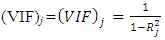Ridge regression technique is based on adding a ridge parameter (λ) to the diagonal of X’X matrix forming a new matrix (X’X+λI). It’s called ridge regression because the diagonal of ones in the correlation matrix can be described as a ridge [6]. The ridge formula to find the coefficients is 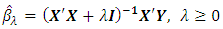. When λ=0, the ridge estimator become as the OLS. If all are the same, the resulting estimators are called the ordinary ridge estimators [14, 15]. It is often convenient to rewrite ridge regression in Lagrangian form:

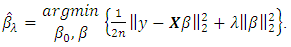Ridge regression has the ability to overcome this multicollinearity by constraining the coefficient estimates, hence, it can reduce the estimator’s variance but introduce some bias [16].

b. The LASSO

The LASSO regression estimates by the optimazation problem:

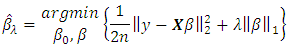for some By Lagrangian duality, there is one-to-one correspondence between constrained problem and the Lagrangian form. For each value of t in the range where the constraint is active, there is a corresponding value of λ that yields the same solution form Lagrangian form. Conversely, the solution of to the problem solves the bound problem with [17, 18].

Like ridge regression, penalizing the absolute values of the coefficients introduces shrinkage towards zero. However, unlike ridge regression, some of the coefficients are shrunken all the way to zero; such solutions, with multiple values that are identically zero, are said to be sparse. The penalty thereby performs a sort of continuous variable selection.

c. Principal Component Regression (PCR)

Let V=[V₁,...,V_p} be the matrix of size p x p whose columns are the normalized eigenvectors of , and let λ₁,..., λ_p be the corresponding eigenvalues. Let W=[W1,...,Wp]= XV. Then W_j= XV_j is the j-th sample principal components of X. The regression model can be written as where . Under this formulation, the least estimator of is

And hence, the principal component estimator of β is defined by 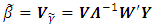[19-21]. Calculation of OLS estimates via principal component regression may be numerically more stable than direct calculation [22]. Severe multicollinearity will be detected as very small eigenvalues. To rid the data of the multicollinearity, principal component omit the components associated with small eigen values.

2.3. Measurement of Performances

To evaluate the performances at the methods studied, Average Mean Square Error (AMSE) of regression coefficient is measured. The AMSE is defined by

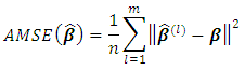where denotes the estimated parameter in the l-th simulation. AMSE value close to zero indicates that the slope and intercept are correctly estimated. In addition, Akaike Information Criterion (AIC) is also used as the performance criterion with formula: 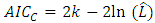where are the parameter values that maximize the likelihood function, x = the observed data, n = the number of data points in x, and k = the number of parameters estimated by the model [23, 24]. The best model is indicated by the lowest values of AIC.

3. Methods

In this study, we consider the true model as . We simulate a set of data with sample size n= 25, 50, 75, 100, 200 contain severe multicolleniarity among all explanatory variables (ρ=0.99) using R package with 100 iterations. Following [25] the explanatory variables are generated by

Where are independent standard normal pseudo-random numbers and ρ is specified so that the theoretical correlation between any two explanatory variables is given by . Dependent variable for each p explanatory variables is from with β parameters vectors are chosen arbitrarily for p= 4, 6, 8, 10, 20 and ε~N (0, 1). To measure the amount of multicolleniarity in the data set, variance inflation factor (VIF) is examined. The performances of OLS, LASSO, RR, and PCR methods are compared based on the value of AMSE and AIC. Cross-validation is used to find a value for the λ value for RR and LASSO.

4. Results and Discussion

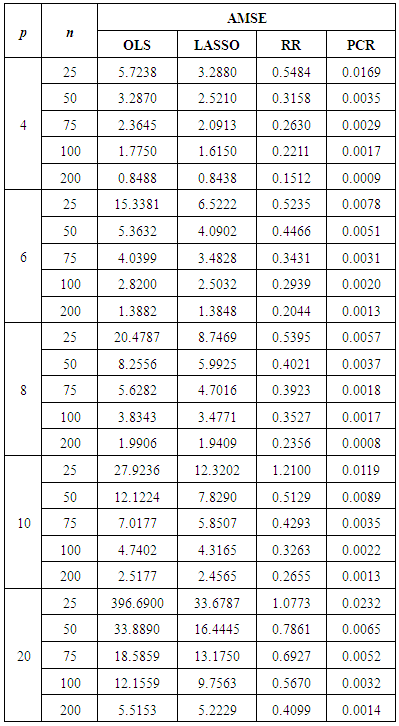
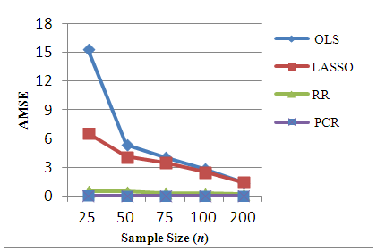
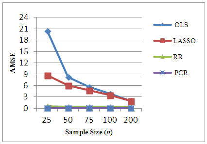
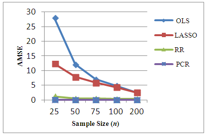
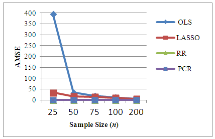
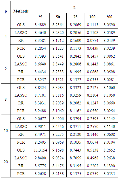
The existence of severe multicollinearity in explanatory variables for all given cases are examined by VIF values. The result of the analysis to simulated dataset with p = 4, 6, 8, 10, 20 with n = 25, 50, 75, 100, 200 gives the VIF values among all the explanatory variables are between 40-110. This indicates that severe multicollinearity among all explanatory variables is present in the simulated data generated from the specified model and that all the regression coefficients appear to be affected by collinearity. LASSO method is for choosing which covariates to include in the model. It is based on stepwise selection procedure. In this study, LASSO, cannot overcome severe multicollinearity among all explanatory variables since it can reduce the VIF in data set a little bit. Whereas in every cases of simulated data set studied, RR reduces the VIF values less than 10 and PCR reduce the VIF to 1. Using this data, we compute different estimation methods alternate to OLS. The experiment is repeated 100 times to get an accurate estimation and AMSE of the estimators are observed. The result of the simulations can be seen in Table 1.

In order to compare the four methods easily, the AMSE results in Table 1 are presented as graphs in Figure 1 - Figure 5. From those figures, it is seen that OLS has the highest AMSE value compared to the other three methods in every cases being studied followed by LASSO. Both OLS and LASSO are not able to resolve the severe multicollinearity problems. On the other hand, RR gives lower AMSE than OLS and LASSO but still high as compare to that in PCR. Ridge regression and PCR seem to improve prediction accuracy by shrinking large regression coefficients in order to reduce over fitting. The lowest AMSE is given by PCR in every case.

Table 1. Average Mean Square Error of OLS, LASSO, RR, and PCR

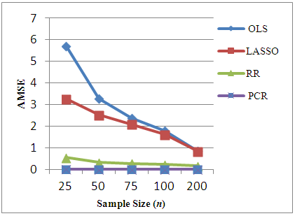Figure 1. AMSE of OLS, LASSO, RR and PCR for p=4

Figure 2. AMSE of OLS, LASSO, RR and PCR for p=6

Figure 3. AMSE of OLS, LASSO, RR and PCR for p=8

Figure 4. AMSE of OLS, LASSO, RR and PCR for p=10

Figure 5. AMSE of OLS, LASSO, RR and PCR for p=20

It clearly indicates that PCR is the most accurate estimator when severe multcollinearity presence. The result also show that sample size affects the value of AMSEs. The higher the sample size used, the lower the value of AMSE from each estimators. Number of explanatory variables does not seem to affect the accuracy of PCR.

To choose the best model, we use Akaike Information Criterion (AIC) of the models obtained using the four methods being studied. The AIC values for all methods with different number of explanatory variables and sample sizes is presented in Table 2 and displayed as bars-graphs in Figure 6 – Figure 10.

Table 2. AIC values for OLS, RR, LASSO, and PCR with different number of explanatory variables and sample sizes

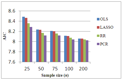Figure 6. Bar-graph of AIC for p=4

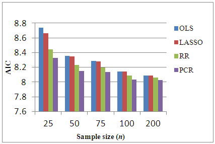Figure 7. Bar-graph of AIC for p=6

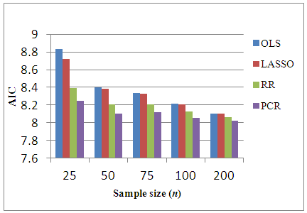Figure 8. Bar-graph of AIC for p=8

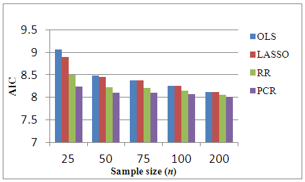Figure 9. Bar-graph of AIC for p=10

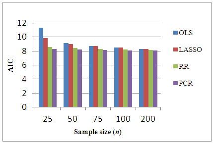Figure 10. Bar-graph of AIC for p=20

Figure 6 –Figure 10 show that the greater the sample sizes are the lower the values of AIC and in contrary to sample sizes, number of explanatory variables does not seem to affect the value of AIC. OLS has the highest AIC values in every level of explanatory variables and sample sizes. LASSO as one of the regularized method has the highest AIC values compare to RR and PCR. The differences of AIC values between the PCR performances from RR are small. PCR is the best methods among the selected methods including based on the value of AIC. It is consistent with the result in Table 1 where PCR has the smallest AMSE value among all the methods applied in the study. PCR is approximately effective and efficient for a small and high number of regressors. This finding is in accordance with previous study [20].

5. Conclusions

Based on the simulation results at p = 4, 6, 8, 10, and 20 and the number of data n = 25, 50, 75, 100 and 200 containing severe multicollinearity among all explanatory variables, it can be concluded that RR and PCR method are capable of overcoming severe multicollinearity problem. In contrary, the LASSO method does not resolve the problem very well when all variables are severely correlated even though LASSO do better than OLS. In Overall PCR performs best to estimate the regression coefficients on data containing severe multicolinearity among all explanatory variables.