-
Paper Information
- Next Paper
- Paper Submission
-
Journal Information
- About This Journal
- Editorial Board
- Current Issue
- Archive
- Author Guidelines
- Contact Us
International Journal of Statistics and Applications
p-ISSN: 2168-5193 e-ISSN: 2168-5215
2018; 8(4): 153-166
doi:10.5923/j.statistics.20180804.01

Spatio-Temporal Analysis of Childhood Malnutrition in Republic of Congo
 Abstract
 Reference
 Full-Text PDF
 Full-text HTML
Owen P. L. Mtambo
Mathematics and Statistics, Namibia University of Science and Technology, Windhoek, Namibia
Correspondence to: Owen P. L. Mtambo, Mathematics and Statistics, Namibia University of Science and Technology, Windhoek, Namibia.
| Email: |  |
Copyright © 2018 The Author(s). Published by Scientific & Academic Publishing.
This work is licensed under the Creative Commons Attribution International License (CC BY).
http://creativecommons.org/licenses/by/4.0/

Background: The pooled prevalence of childhood overweight and obesity worldwide dramatically increased between 2000 and 2013. If these increasing trends continue, it is estimated that the prevalence of overweight (including obesity) in children under 5 years of age will rise to 11% worldwide by 2025, up from 7% in 2012 [1, 9]. Research has shown that the pooled prevalence of overweight (including obesity) among children under five years in sub-Saharan Africa was about 5% in 2012 and is expected to reach about 8% by 2025 [1, 9, 38]. The pooled prevalence of stunting among children under five years in sub-Saharan Africa was about 43% in 2000 and about 34% in 2016. [1, 8] To reduce childhood malnutrition, several interventions including scaling-up nutrition programmes are currently operational in most sub-Saharan African countries including Republic of Congo [2]. However, very few studies have ever fitted in-depth statistical models for childhood malnutrition in Republic of Congo. The main objective of this study was to fit newly proposed spatio-temporal quantile interval regression models for childhood stunting, overweight, and obesity in Republic of Congo from 2005 to 2012. Methods: The Demographic and Health Survey (DHS) datasets for Republic of Congo from 2005 to 2012 were used in this study. The spatio-temporal quantile interval regression models were used to analyse childhood stunting, overweight, and obesity in Republic of Congo from 2005 to 2012. The statistical inference performed in this study was fully Bayesian using R-INLA package [37, 38] implemented in R version 3.4 [39]. Results: We observed that significant determinants of childhood malnutrition ranged from socio-demographic factors to child and maternal factors. In addition, child age and preceding birth interval had significant nonlinear effects on childhood stunting, overweight, and obesity. Furthermore, mother’s body mass index had significant nonlinear effects on childhood overweight and obesity. Lastly, I also observed significant spatial and temporal effects on childhood stunting, overweight, and obesity in Republic of Congo. Conclusions: To achieve the World Health Organisation (WHO) global nutrition targets 2025 in Republic of Congo [8, 9], scaling-up nutrition programmes and childhood malnutrition policy makers should consider timely interventions based on socio-demographic determinants and spatial targets as identified in this paper.
Keywords: Bayesian inference, Spatio-temporal model, Quantile interval regression, R-INLA, Childhood malnutrition, Childhood stunting, Childhood overweight, Childhood obesity
Cite this paper: Owen P. L. Mtambo, Spatio-Temporal Analysis of Childhood Malnutrition in Republic of Congo, International Journal of Statistics and Applications, Vol. 8 No. 4, 2018, pp. 153-166. doi: 10.5923/j.statistics.20180804.01.
Article Outline
1. Background
- Childhood malnutrition has severe adverse effects on the growth of any child and the economy of any nation. The most common indicators of childhood malnutrition are stunting, wasting, underweight, overweight, and obesity. A malnourished child is more likely to fall sick and die [3]. In sub-Saharan Africa, malnutrition often leads to more than 30% of deaths in children below five years annually [4]. Malnutrition is also a strong indicator of retarded growth [5], impaired cognitive and behaviour development [6], poor school performance, and lower working capacity [7]. If not corrected, it can slow down economic growth and increase poverty levels. Furthermore, it can prevent a nation from meeting its full potential through loss in productivity, cognitive capacity and increased cost in health care [6]. The prevalence of childhood overweight and obesity worldwide dramatically increased between 2000 and 2013. If these increasing trends continue, it is estimated that the prevalence of overweight (including obesity) in children under 5 years of age will rise to 11% worldwide by 2025, up from 7% in 2012 [1, 9]. The prevalence of stunting among children under five years in sub-Saharan Africa was about 43% in 2000 and about 34% in 2016 [1, 8]. Doubly surprising, childhood overnutrition is alarmingly becoming more prevalent parallel to existing undernutrition burden in sub-Saharan Africa. The prevalence of overweight (including obesity) among children under five years in sub-Saharan Africa was about 5% in 2012 and is expected to reach about 8% by 2025 [1, 9, 36].The consequences of overnutrition can be more devastating than those for undernutrition because it leads to chronic failure problems which in turn lead to increased medical expenditure. Children who are either overweight or obese are at a higher risk of developing serious health problems, including type 2 diabetes, high blood pressure, asthma and other respiratory problems, sleep disorders and liver disease. They may also suffer from psychological effects, such as low self-esteem, depression and social isolation. Childhood overweight and obesity also increase the risk of obesity, noncommunicable diseases (NCD), premature death and disability in adulthood. Finally, the economic costs of the escalating problem of childhood overweight and obesity are considerable, both in terms of the enormous financial strains it places on health-care systems and in terms of lost economic productivity [9].The overall WHO global nutrition target 2025 is to improve maternal, infant and young child nutrition. One of the specific nutrition targets is the stunting policy which aims at reduction of childhood stunting by 40% from 2014 to 2025 [8]. Another specific nutrition target is the overweight (including obesity) policy which aims at making sure that there is no more increase in prevalence of childhood overweight from 2014 to 2025 [9]. To attain these targets, various malnutrition interventions including scaling-up nutrition programmes are available in most sub-Saharan African countries including Republic of Congo [2]. However, very few studies have ever fitted in-depth statistical models for childhood stunting in Republic of Congo. The main aim of this study was to assess socio-demographic determinants and spatio-temporal variation of childhood stunting, overweight, and obesity in Republic of Congo from 2005 to 2012 using newly proposed spatio-temporal quantile interval regression models and R-INLA package [37, 38] implemented in R version 3.4 [39].Spatial models have previously been used to analyse childhood malnutrition in most sub-Saharan African countries [11, 12, 40, 41, 42]. Unfortunately, most of them have emphasised on modeling mean regression instead of quantile regression. Modeling malnutrition using quantile regression is more appropriate than using mean regression with extensive literature examples [13, 14, 15, 20, 25, 26, 27, 28, 29, 30, 43] in that it provides flexibility to analyse the determinants of malnutrition corresponding to quantiles of interest either in the lower tail (say 5% or 10%), upper tail (say 90% or 95%) or even median (50%) of the distribution rather than only analysing the determinants of mean distribution. When modeling malnutrition, it makes more sense to model severe responses rather mean responses [13, 14, 15, 20, 25, 26, 27, 28, 29, 30, 43]. For instance, it is more sensible to model severe stunting or severe overweight/obesity which corresponds to the lower and upper tails of the distribution of the same anthropometric measure than to model mean stunting or mean overweight/obesity which corresponds to the average nutritional response.Furthermore, almost all studies on quantile modeling have emphasised on selecting only one specific response quantile level of interest and report the recommendations based on the only chosen response quantile. Unlike mean response modeling, quantile regression yields model estimates which are stochastic functions of quantiles
 such that
  This implies that quantile regression modeling using estimates based on only one chosen quantile level
  might be insufficient and not robust enough. In this study, I proposed a new quantile interval modeling approach which is sufficient and robust because it uses weighted mean estimates based on all quantile levels in a specified quantile interval
  of interest.
2. Materials and Methods
- This section summarises the conceptual framework of the spatio-temporal quantile interval regression models, the data sources, and data analysis procedures used in this study. Quantile Regression ModelIn general, quantile regression is about describing conditional quantiles of the response variable in terms of covariates instead of the mean. The general additive conditional quantile model is given by
 | (1) |
 is the conditional
  quantile response given
  and
and  is the semi-parametric predictor,
  is the
  quantile of the response e.g.
  for the median response regression,
  is the vector of p categorical covariates (assumed to have fixed effects) for each individual i,
  is the vector of q metric/spatial/temporal covariates,
  is the vector of p coefficients for categorical covariates at a given
  ,
,  is the vector of q smoothing functions for metric/spatial/temporal covariates at a given
  [13, 14, 26]. It is worthy to note that quantile regression duplicates the roles of median, tertile, quartile, quintile, sextile, septile, octile, decile, hexadecile, duodecile, ventile, percentile, and permille regressions. This is achieved by selecting appropriate values of
  in the conditional quantile regression model where
  .The two unknowns,
  and
and  are estimated via the minimization rule given by
 | (2) |
 is the check function (appropriate loss function) evaluated at a given
  ,
,  is the zeroth (initial) tuning parameter for controlling the smoothness of the estimated function,
  is the
  tuning parameter for controlling the smoothness of the estimated function,
  and
and  denotes the total variation of the derivative on the gradient of the function
  [13, 15, 16].Proposed Quantile Interval Regression EstimationLet the quantile interval
  be of interest where
  is the desired quantile interval median of interest and
  is the desired quantile bandwidth. I propose a new methodology for estimating the quantile interval weighted mean estimates for
  fixed effects parameters denoted by
  for
for  and q nonlinear/spatio-temporal effects smoothing functions denoted by
  for
for  in three steps as follows. Step 1: Divide the quantile interval
  into n equally spaced subintervals with a uniform step size of
  such that
  is a positive even integer. This step ensures that I have discretized the quantile interval
  into
into  odd number of equally spaced quantiles denoted by quantile set
  such that
  , and
, and  . The step size h is supposed to be determined by the user in such a way that it is small enough relative to the bandwidth
  . Since it is more natural to use percentiles, I propose a default step size of
  .Step 2: For each
  of the
  fixed effects parameters, compute all
  quantile estimates
  where
where 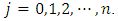 Similarly, for each
  of the q nonlinear/spatio-temporal effects smoothing functions, compute all
  quantile estimates
  where
where 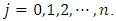 Step 3:Compute the quantile interval weighted mean estimates for
  fixed effects parameters denoted by
  for each
  using the formula
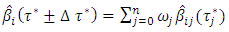 | (3) |
 normalized j-th weight assigned to
  such that
  Similarly, compute the quantile interval weighted mean estimates for q nonlinear/spatio-temporal effects smoothing functions denoted by
 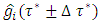 for each
  using the formula
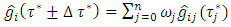 | (4) |
 normalized j-th weight assigned to
  such that
  The normalized weights
  are supposed to be determined by the user basing on application at hand. For simplicity, I proposed a default of equal weights
  for each
  which consequently corresponds to quantile interval equally weighted mean estimates (or simply quantile interval mean estimates) as follows.
 | (5) |
 | (6) |
 i.e.
i.e.  where
where  was the desired quantile interval median of interest and
  was the desired quantile bandwidth.For childhood overweight, the primary interest was to model the childhood body mass index-for-age Z-score (BMIAZ) in the quantile interval
  i.e.
i.e.  where
where  was the desired quantile interval median of interest and
  was the desired quantile bandwidth.For childhood obesity, the primary interest was to model the childhood body mass index-for-age Z-score (BMIAZ) in the quantile interval
  i.e.
i.e.  where
where  was the desired quantile interval median of interest and
  was the desired quantile bandwidth.Prior DistributionsIn fully Bayesian framework, all unknown functions
  for both metric and spatio-temporal covariates, all parameters
  for categorical covariates, and all variance parameters
  are considered as random variables and must be supplemented by appropriate prior distributions. In this research, the following prior distributions were supplemented. The priors for unknown functions
  do belong to the class of Gaussian Markov random fields (GMRF), whose specific forms actually depend on covariate types and also on the prior beliefs about the smoothness of
  . Although only GMRF was used in this study, there exist some other options like Bayesian P-splines [15, 17].Let
  , a random vector of the response at
  The vector
  is a GMRF with mean
  and precision (the inverse covariance) matrix
  if and only if it has density of form
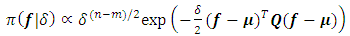 | (7) |
 where
where  The properties of a particular GMRF are all reflected through matrix Q. For instance, the Markov properties of GMRFs totally depend on the various sparse structures that the matrix Q may have. In this paper, I used two kinds of GMRFs: second order random walk (RW2) models [18] for metric covariates and intrinsic conditional autoregressive (ICAR) models [19] for spatial covariates. These two GMRFs share equation 7 but with different structures of Q.For metric covariates, let
  be the set of continuous locations and
  be the function evaluations at
  for
for  Then construction of RW2 model is based on a discretely observed continuous time process
  that is a realization of an
  fold integrated Wiener process given by
 | (8) |
 is a standard Wiener process.For spatial covariates, letting
  denote the number of neighbours of site
  I assumed the following spatial smoothness prior for the function evaluations
 | (9) |
 denotes that site
  and
and  are neighbors. Thus, the conditional mean of
  is an un-weighted average of evaluations of neighbouring sites.For the fixed effect parameters
  I assumed independent diffuse priors
  constant or a weakly informative Gaussian
  with small precision
  on the identity matrix I. If
  is a high-dimensional vector, one may consider using Bayesian regularization priors developed in [17], where conditionally Gaussian priors are assigned with suitable hyper prior assumptions on the variances inducing the desired shrinkage and sparseness on coefficient estimates.Spatio-temporal modelsThe spatio-temporal data can be defined by a stochastic process
  and are observable or measurable at n spatial locations or areas and at given T time points. Since the space and time dimensions are always correlated, a valid spatio-temporal covariance function given as
  must always be defined and assessed [31, 44]. If an assumption of stationarity in space and time is made, then the space-time covariance function can simply be written as a function of both the spatial Euclidean distance
  and the temporal lag
  , as
, as  . Note that many valid non-separable space-time covariance functions are also possible as are reported in [32].To overcome the computational complexity of non-separable models, many simplifications have been introduced in practice. For instance, basing on the separability hypothesis, the space-time covariance function can be decomposed into either sum or the product of a purely spatial component and a purely temporal component, e.g.
 , as described in [33]. In some cases, it is also possible to assume that the spatial correlation is constant over time so that a space-time covariance function becomes purely spatial when
  i.e.
i.e.  , and is zero otherwise. Consequently, the temporal evolution can also be introduced with an assumption that the spatial process evolves with time following some autoregressive dynamics [34]. Similarly, the GMRF framework for area level spatio-temporal data analysis can be extended to include a precision matrix that is defined also in terms of time with a neighbourhood structure assumption. It is worthy to note that if a space-time interaction is included, then its precision can be obtained through the Kronecker product of the precision matrices for the space and time effects interacting [35].In this research, I performed spatio-temporal data analysis of childhood stunting, overweight, and obesity in Republic of Congo. In this case, the datasets were defined by stochastic processes of the form
  where
where  were childhood height-for-age Z-score (HAZ) and childhood body mass index-for-age Z-score (BMIAZ) as a continuous response variable at a given 2-dimensional (latitude and longitude) spatial location s which was a region of Republic of Congo at a given time point (year) T which ranged from 2005 to 2012. For simplicity, I assumed stationarity in space and time to easily decompose the space-time covariance function into a sum or product of purely spatial and purely temporal terms.Posterior InferenceThe well-known method for estimating Bayesian posterior marginal distribution is Markov chain Monte Carlo (MCMC). The alternative method is Integrated Nested Laplace Approximations (INLA). In this study, INLA method was used because it is generally faster than MCMC for quantile models [21, 22, 23, 24, 37, 38, 45]. Data SourcesFor applications of the newly proposed methodology, I considered the Demographic and Health Survey (DHS) datasets of Republic of Congo from 2005 to 2012. A multi-stage clustered sampling technique was used to interview eligible women of reproductive age between 15 and 49 years. The anthropometric assessment of themselves and their children that were born within the previous 5 years preceding the survey were administered. These DHS datasets contained information on family planning, maternal and child health, child survival, educational attainment, and other household composition and characteristics.Data AnalysisFirstly, I started with estimating the crude prevalence rates of childhood stunting, overweight, and obesity in the Republic of Congo from 2005 to 2012. The categorized adjusted childhood stunting with two categories, stunted
  and not stunted (otherwise), was used as a childhood stunting indicator variable in this phase. The categorized adjusted childhood overweight with two categories, overweight
  and not overweight (otherwise), was used as a childhood overweight indicator variable in this phase. The categorized adjusted childhood obesity with two categories, obese
  and not obese (otherwise), was used as a childhood obesity indicator variable in this phase.Finally, I performed spatio-temporal data analysis of childhood malnutrition in Republic of Congo from 2005 to 2012. The primary outcomes in this study were the childhood (under 5 years) stunting, overweight, and obesity in Republic of Congo from 2005 to 2012. On one hand, childhood stunting was assessed by using the childhood height for age Z-score (HAZ) as a continuous response variable. On the other hand, childhood overweight and obesity were assessed by body mass index-for-age Z-score (BMIAZ) as a continuous response variable. The statistical inference was fully Bayesian using the newly proposed quantile interval estimation approach and INLA approach implemented in R version 3.4 with reference to examples cited in [21, 22, 23, 24, 37, 38, 45].
3. Results
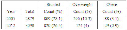
- Firstly, the exploratory results were assessed in terms of trends in crude prevalence rates of stunting, overweight, and obesity in Republic of Congo from 2005 to 2012. Secondly, the results of spatio-temporal quantile interval regression models were assessed in terms of fixed effects, nonlinear effects, and spatial effects.Prevalence of Childhood MalnutritionTable 1 and Figure 1 show the trends in prevalence rates for childhood stunting, overweight, and obesity in Republic of Congo from 2005 to 2012. Firstly, the prevalence of childhood stunting in Republic of Congo slightly decreased from 28.1% in 2005 to 26.5% in 2012. Secondly, the prevalence of childhood overweight in Republic of Congo decreased from 10.3% in 2005 to 4% in 2012. Lastly, the prevalence of childhood obesity in Republic of Congo also decreased from 3.1% in 2005 to 0.9% in 2012.
|
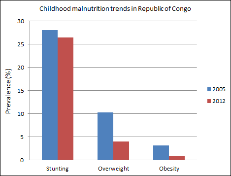 | Figure 1. Trends of childhood malnutrition prevalence rates in Republic of Congo |
|
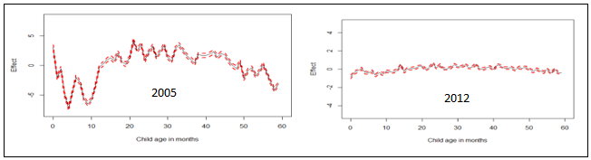
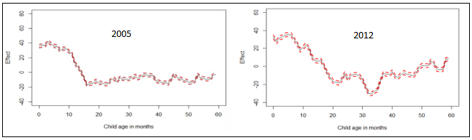 | Figure 2. Nonlinear effects of child’s age in months on childhood stunting in Republic of Congo |
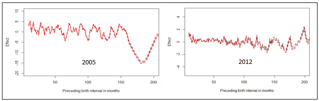
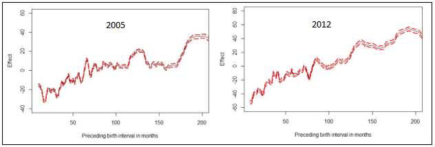 | Figure 3. Nonlinear effects of preceding birth interval in months on childhood stunting in Republic of Congo |
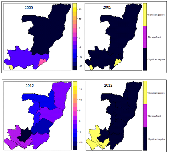 | Figure 4. Spatial effects on childhood stunting: posterior means (left); significance at 95% level (right) |
|
 | Figure 5. Nonlinear effects of child’s age in months on childhood overweight in Republic of Congo |
 | Figure 6. Nonlinear effects of preceding birth interval in months on childhood overweight in Republic of Congo |
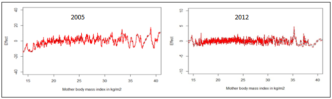 | Figure 7. Nonlinear effects of mother’s BMI in kg/m2 on childhood overweight in Republic of Congo |
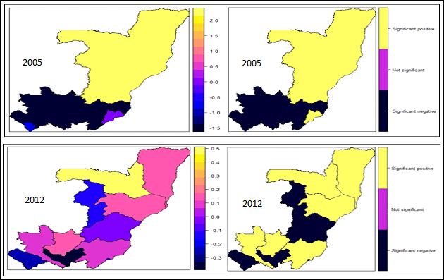 | Figure 8. Spatial effects on childhood overweight: posterior means (left); significance at 95% level (right) |
|

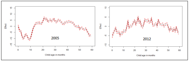 | Figure 9. Nonlinear effects of child’s age in months on childhood obesity in Republic of Congo |
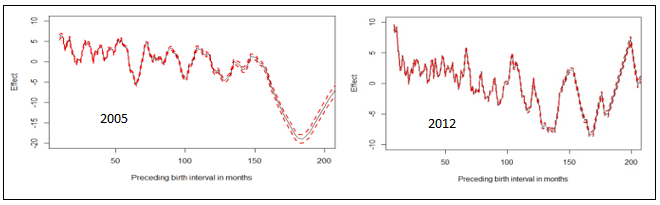 | Figure 10. Nonlinear effects of preceding birth interval in months on childhood obesity in Republic of Congo |
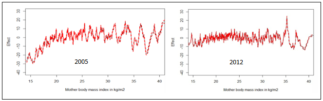 | Figure 11. Nonlinear effects of mother’s BMI in on childhood obesity in Republic of Congo |
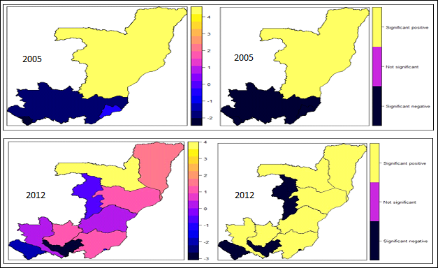 | Figure 12. Spatial effects on childhood obesity: posterior means (left); significance at 95% level (right) |
4. Discussion
- In this study, the spatio-temporal quantile interval regression models were fitted for childhood stunting, overweight, and obesity using the newly proposed weighted mean estimation for the first time. The indicators of childhood undernutrition are stunting, wasting and underweight. However, only childhood stunting was assessed in this study because it has always been the most prevalent undernutrition status among children under-five in sub-Saharan Africa [1, 4]. The indicators of childhood overnutrition are overweight and obesity. Note that I managed to analyse both in this study.The primary aim of this study was to fit country-specific spatio-temporal quantile interval models in Republic of Congo which are more appropriate than mean regression models when modeling nutritional status.For childhood stunting, I analysed the height-for-age Z-scores (HAZ) in the quantile interval
 i.e.
i.e.  where
where  was the desired quantile interval median of interest and
  was the desired quantile bandwidth.For childhood overweight, I analysed the childhood body mass index-for-age Z-score (BMIAZ) in the quantile interval
  i.e.
i.e.  where
where  was the desired quantile interval median of interest and
  was the desired quantile bandwidth.For childhood obesity, I analysed the childhood body mass index-for-age Z-score (BMIAZ) in the quantile interval
  i.e.
i.e.  where
where  was the desired quantile interval median of interest and
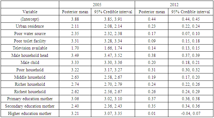
  was the desired quantile bandwidth.The inference used in this study was fully Bayesian. The posterior marginal distributions were estimated using R-INLA package [37, 38] in R version 3.4 [39]. The INLA approach was chosen because it is generally faster than MCMC approach for quantile models [23, 27].Despite a few minor differences in terms of statistical approaches, most of the findings in this study were very similar to those reported in most related studies in sub-Saharan Africa [11, 12, 40, 41, 42]. For example, childhood stunting was analysed in two sub-Saharan African countries; Tanzania and Zambia in 2005 using 1992 DHS datasets [11] and childhood stunting was analysed in Nigeria in 2008 using the 2005 DHS dataset [12]. They both also found that rural residence, poor source of drinking water, poor type of toilet facility, male-headed household, male child, higher household wealth index, and lower mother’s formal education were significantly associated with increased childhood stunting in these countries. Furthermore, all of them also observed U-shaped patterns of nonlinear effects of child's age on childhood stunting which was the same finding I observed in our study.However, a few differences are as follows. Firstly, they used MCMC simulation techniques to estimate the posterior mean effects whereas I used INLA direct computation techniques to estimate the posterior mean effects. Secondly, they analysed mean responses of childhood stunting by using Bayesian semi-parametric geo-additive models whereas I analysed quantile interval responses of childhood stunting in the quantile interval
  by using Bayesian spatio-temporal quantile interval models. Note that my approach is more appropriate than their approaches because it is more appropriate to model severe childhood stunting than to model the average childhood stunting.
5. Conclusions
- The prevalence of childhood stunting in Republic of Congo, though still considerably high, decreased from 28.1% in 2005 to 26.5% in 2012. The prevalence of overweight decreased from 10.3% in 2005 to 4% in 2012. Similarly, the prevalence of overweight also decreased from 3.1% in 2005 to 0.9% in 2012.In general, I found that rural residence, poor source of drinking water, poor type of toilet facility, male-headed household, male child, higher household wealth index, and lower mother’s formal education were significantly associated with increased childhood stunting in Republic of Congo from 2000 to 2012.I observed that urban residence, poor source of drinking water, poor type of toilet facility, availability of TV, male-headed household, and male child significantly increased childhood overweight and obesity in Republic of Congo over the period from 2005 to 2012. In addition, richer households were associated with reduced childhood overweight and obesity compared to poor households. Furthermore, households with highly educated mothers (graduates) were associated with lower prevalence rates of childhood overweight and obesity compared to households with less educated mothers (secondary or below) in Republic of Congo in 2012.In general, it was observed that childhood stunting, overweight, and obesity increased as age of child increased whereas childhood stunting, overweight, and obesity decreased as preceding birth interval increased. I also found out that childhood overweight and obesity increased as mother’s BMIs increased. Finally, I noticed that most of the regions exhibited significant spatial effects on childhood stunting, overweight, and obesity in Republic of Congo from 2005 to 2012.I recommend that scaling-up nutrition programmes, food security programmes, and childhood malnutrition policy makers should consider timely interventions based on important socio-demographic factors, child age, maternal factors, temporal and spatial variation of childhood stunting, overweight, and obesity in Republic of Congo as reported in this paper.
List of Abbreviations
- BMI: Body mass index; BMIAZ: Body mass index-for-age Z-score; DHS: Demographic and health survey; GMRF: Gaussian Markov random field; HAZ: Height-for-age Z-score; ICAR: Intrinsic conditional autoregressive; INLA: Integrated nested Laplace approximations; MCMC: Markov chain Monte Carlo; NCD: Non-communicable diseases; RW2: Random walk order 2; SUN: Scaling up nutrition; TV: Television; UNICEF: United nations children’s fund; WFP: World food programme; WHO: World health organisation
ACKNOWLEDGEMENTS
- Firstly, I acknowledge the permission granted by Measure DHS to use the DHS datasets for Republic of Congo from 2005 to 2012. Lastly, I would like to thank all anonymous peer reviewers for their scrutiny of the original manuscript.