-
Paper Information
- Previous Paper
- Paper Submission
-
Journal Information
- About This Journal
- Editorial Board
- Current Issue
- Archive
- Author Guidelines
- Contact Us
International Journal of Statistics and Applications
p-ISSN: 2168-5193 e-ISSN: 2168-5215
2018; 8(3): 144-152
doi:10.5923/j.statistics.20180803.05

An Empirical Comparison of Principal Component Analysis and Clustering on Variables for Dimension Reduction Using Leukemia and Breast Cancer Data
 Abstract
 Reference
 Full-Text PDF
 Full-text HTML
Khaled I. A. Almaghri1, S. Chakraborty2
1Pharmacology College, Palestine University, Gaza, Palestine
2Department of Statistics, Dibrugarh University, Assam, India
Correspondence to: Khaled I. A. Almaghri, Pharmacology College, Palestine University, Gaza, Palestine.
| Email: |  |
Copyright © 2018 The Author(s). Published by Scientific & Academic Publishing.
This work is licensed under the Creative Commons Attribution International License (CC BY).
http://creativecommons.org/licenses/by/4.0/

One of the important problems of data analysis is that identifying nuisance variable(s) in a data set that contributes to an increase of variability within groups in an experiment. One way to address this issue is through dimension reduction of data sets. In this study we compare between two widely used methods of reducing dimension data sets, namely the method of the principal component (PC), statistics technical that uses orthogonal transformation to convert a set of possibly correlated variables of into a new set of uncorrelated variables and the method of clustering on variables, where the aim is to put the variables with similar information in the same group or cluster by considering two celebrated data sets from literature, the leukemia dataset and the other a breast cancer data.
Keywords: Acute lymphoblastic leukemia "ALL", Breast cancer, Clustering on variables, Dimension reduction, Scree plot, Correlation matrix, Cumulative variance proportion, Principal component analysis
Cite this paper: Khaled I. A. Almaghri, S. Chakraborty, An Empirical Comparison of Principal Component Analysis and Clustering on Variables for Dimension Reduction Using Leukemia and Breast Cancer Data, International Journal of Statistics and Applications, Vol. 8 No. 3, 2018, pp. 144-152. doi: 10.5923/j.statistics.20180803.05.
Article Outline
1. Introduction
- In biostatistics data set with higher dimension is often difficult to handle and may cause waste of time. Principal component analysis (Sanche and Lonergan, 2006 [14], (pp.439, Izenman, 2008 [7])) is a useful statistical techniques to reduce dimension but at the cost of loosing of information. Clustering on variables is used to construct clusters of homogenous variables so that we can choose one representative variable from each cluster for using in our model or statistical analysis without losing any information. The later method also allow us to avoid those variables in a clusters which need more time to for observation and hence more time in data collection.
2. Material and Methods
2.1. Acute Lymphoblastic Leukemia (ALL) Data Set
- Acute Lymphoblastic Leukemia data set taken from Ritz Laboratory (Everitt et al., 2004 [3]) consists of micro arrays from 128 different individuals with acute lymphoblastic leukemia (ALL). The data available in R database have already been normalized using Robust Multichip Average (rma) (R manual documentation, 2012 [12], Irizarry et al., 2003 [6]). This data frame contains observations on: (i) Patient IDs, (ii) Date of diagnosis, (iii) Sex of the patient (sex), (iv) Age of the patient in years (age), (v) Type and stage of the disease: 'B' indicates B-cell ALL while 'T' indicates T-cell ALL (BT), (vi) ‘Remission’: a factor with two levels, either 'CR' indicates that remission was achieved or 'REF' indicating that the patient was refractory, and remission was not achieved (remission), (vii) ‘CR’: a vector with the following values: 1: “CR”, remission; achieved; 2: “DEATH IN CR”, patient died while in remission; 3: “DEATH IN INDUCTION”, patient died while in induction therapy; 4: “REF”, patient was refractory to therapy (CR), (viii) the date on which remission was achieved, (ix) a logical vector indicating whether t (4; 11) translocation was detected (t411), (x) a logical vector indicating whether t (9; 22) translocation was detected (t922), (xi) a vector indicating the various cytogenetic abnormalities that were detected (cyton), (xii) the assigned molecular biology of the cancer (molb), (xiii) Fusion protein for those with BCR\/ABL which of the fusion proteins was detected, ‘p190’, 'p190\/p210', 'p210' (fusionp), (xiv) the patient’s response to multidrug resistance, either 'NEG', or 'POS' (mdr), (xv) 'kinet' ploidy, either diploid or hyperd (kinet), (xvi) a vector indicating whether the patient had neither continuous complete remission nor not (ccr), (xvii) a vector indicating whether the patient had relapse or not (relapse), (xviii) a vector indicating whether the patient receive a bone marrow transplant or not (transplant), and (xix) follow-up data with 10 possible value 1 to 10 (f.u). The possible values of fu are:1. “AUBMT \/ REL”: autologous bone marrow transplant and subsequent relapse, 2. “BMT \/ CCR”: allogeneic bone marrow transplant and still in continuous complete remission,3. “BMT \/ DEATH IN CR”: after allogeneic bone marrow transplant patient died without relapsing,4. “BMT \/ REL”: after allogeneic bone marrow transplant patient relapsed, 5. “CCR”: patient was in continuous complete remission,6. “CCR \/ OFF”: patient was in continuous complete remission but off-protocol for some reasons,7. “DEATH IN CR”: died when in complete remission, 8. “MUD \/ DEATH IN CR”: unrelated allogeneic bone marrow transplant and death without relapsing,9. “REL”: relapse, and10. “REL \/ SNC”: relapse occurred at central nervous system,The last variable is (xx) a logical vector indicating whether the cytogenesis was normal (citog).The data have been presented in the form of an 'exprSet' object which is suitable for implementation and comparison in many of clusters algorithms (Kumar and Sharma, 2011 [10]; Jonathan et al., 2010 [8]) because one can extract subsets from this dataset as Acute Lymphoblastic Leukemia caused by different causes like T.cells, B.cells. The variable BT gives information about the type (B or T) and stages of the disease (five stages for each type). So from the ALL data set two distinct subsets with respect to two covariates namely T cells and B cells have been extracted for independent investigation using the clustering algorithms.The values of the all the variables in the 95th and the 128th rows of the data set are missing. As such effectively, the ALL dataset comprises observations of 126 individuals, more over in the present work four variables namely the variables Patient IDs, date of diagnosis, age of the patient in years and date on which remission was achieved have been omitted before the analysis as they are not relevant for the present investigation. Therefore, in the current work, 126 observations (rows) with only 16 out of 20 variables have been considered for the analysis.
2.2. Breast Cancer Data
- This dataset is from German Breast Cancer Study Group 2 (Schumacher et al., 1994 [17]; Sauerbrei and Royston, 1999 [16]). This data frame contains the observations on (i) hormonal therapy, a factor at two levels no and yes (ii) age of the patients in years (iii) menopausal status, a factor at two levels pre (premenopausal) and post (postmenopausal) (iv) tumor size (in mm), (v) tumor grade, a ordered factor at levels I < II < III, (vi) number of positive nodes, (vii) progesterone receptor (in fmol) (viii) recurrence free survival time (in days) and (ix) censoring indicator (0- censored, 1- event) of 686 women.
2.3. Dimension Reduction
- (Sanche and Lonergan, 2006 [14], (pp.439, Izenman, 2008 [7]))
2.3.1. Principal Component Analysis
- It is a statistical procedure to transform a set of observations of correlated variables to a set of a linearity uncorrelated variables by orthogonal transformation. We can explain the variance covariance structure of these variables by some of these linear combinations of the original variables.
2.3.2. Cluster Analysis
- Cluster analysis has been used as a tool to overcome the difficulties in handling big data by partitioning the data into a number of interesting clusters and concentrating only on the interesting clusters instead of full data set (Halkidi et al., 2001 [5]).Clustering of the variables is same as those of clustering of objects, where instead of observations, the variables are grouped into homogeneous clusters, that is variables in each cluster will be strongly related to each other and contain same information. As a result one can reduce the dimension of the data by choosing only one representative variable from each of the homogenous clusters. Dimension reduction through clustering of variables can be implemented by using the pvclust and also ClustOfVar packages of R.In the proposed work we used ClustOfVar package by using a bootstrap resampling (50 replications) and plot the stability criterion according to the number of clusters which can help to choice a sensible and suitable number of clusters. [12]
3. Previous Studies
- San and Lowrence (2000 [15]), they conduct a study to introduce locally linear embedded algorithm that computes low dimensional neighbor hood preserving embeddings of high dimensional inputs and they implement it on nonlinear manifolds such as those generated by images of faces or documents of test and they found that their algorithm is more useful.Chris and He (2004 [2]) conducted a study to test the effect of dimension reduction on K-means clustering by using principal component analysis to reduce the data from the original 1000 dimension to 40, 20, 10, 6 and 5 dimensions respectively on 4029 of Gene expression of 96 tissue samples on human Lymphoma. They have applied K-means on 10 random samples of each new groups combination [40, 20, 10, 6 and 5 dimensions], they found that the results systematically and significant were improved. Chris and Tao (2007 [1]) conducted a study to combine linear discriminant analysis (LDA) and K-means clustering and tested this new method on a wide range of datasets for adaptive dimension reduction. They found that this new clustering process subspace selection process. And the learning algorithm performs data clustering and subspace selection simultaneously. They further show that this new algorithm is more effective than other methods of dimension reduction. Shuiwang and Jeieping (2009 [18]) they conduct a study to reduce dimension in Multi-label classification and they compare between least squares loss and hinge loss and they found that the relative performance of formulation with orthonormal transformation and orthonormal features is different for different datasets.Gowrilaksshmi (2011 [4]) conducted a study to use methods for dimension reduction using a combination of principal component and with K-means and Locally Linear Embedding (LLE) combined with K-means and found that all the clustering methods were affected by data dimension reduction and data characteristics such as overlapping between clusters and the presence of noise.Murillo J. and Rodriguez A. (2012 [11]) they conduct a study to study the effect of dimension reduction and data set and they found that reduce of dimension is useful for diminishing the error of probability of classifiers.
4. Results and Observations
4.1. Breast Cancer Data
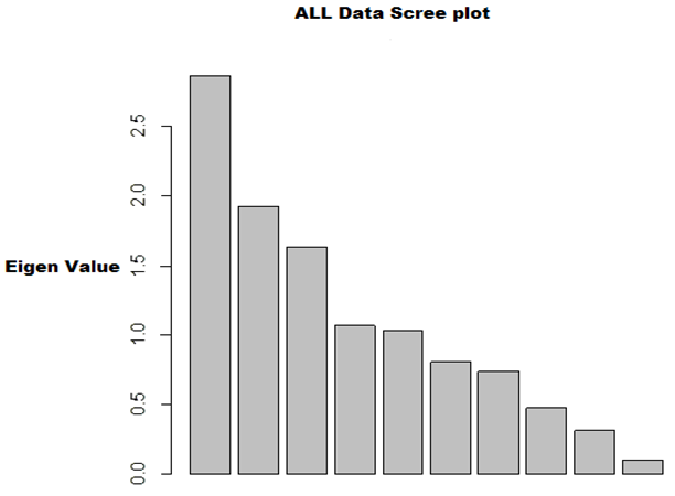
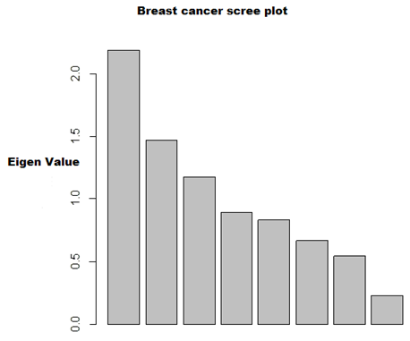 | Figure 1. Scree plot for Breast cancer data |
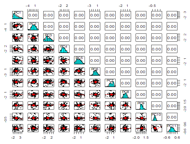
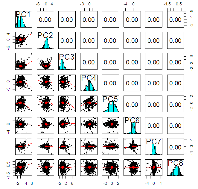 | Figure 2. Correlation matrix between principal components for Breast Cancer data |
|
|
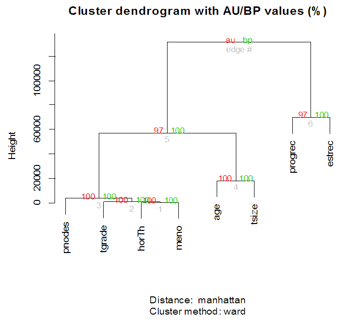 | Figure 3. Clustering on variables for Breast cancer data |
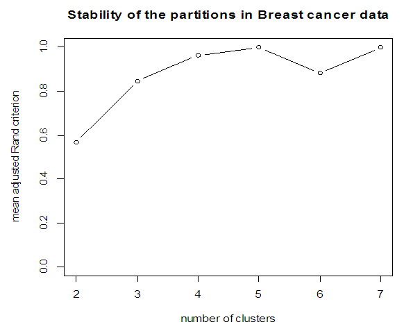 | Figure 4. Stability of partition for Breast cancer data |
 | Figure 5. Scree plot for ALL data |
 | Figure 6. Correlation matrix between principal components for ALL data |
|
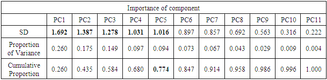
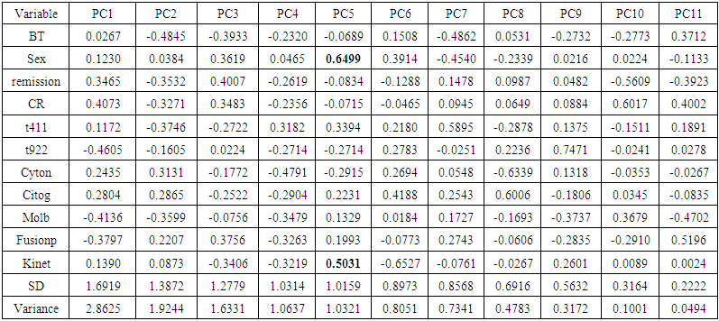 | Table 4. Rotation matrix for Principal component analysis for ALL data |
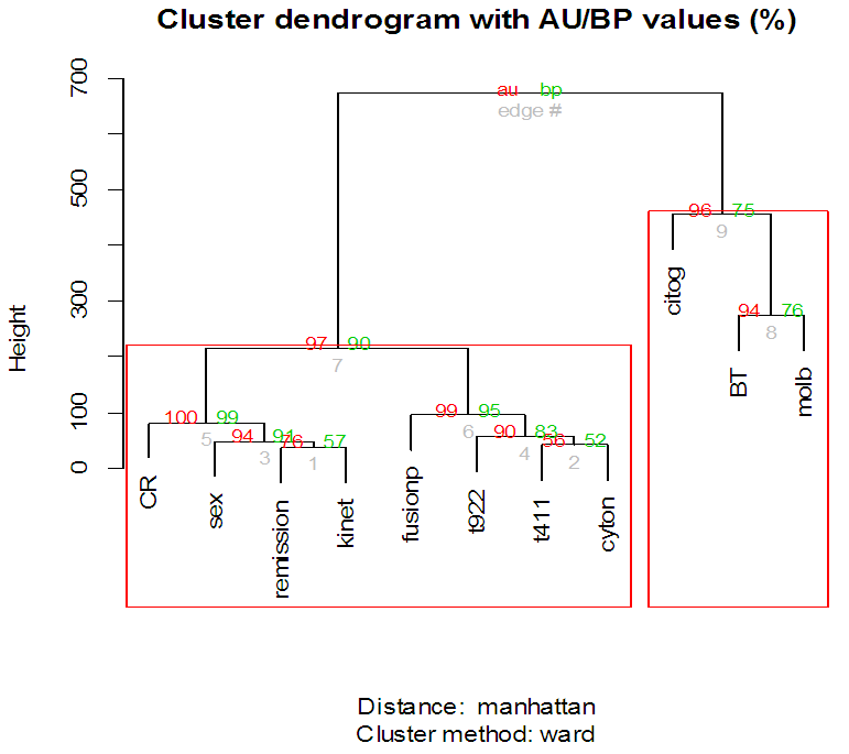 | Figure 7. Clustering on variables for ALL data |
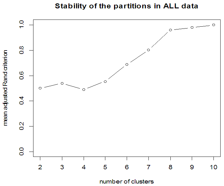 | Figure 8. Stability of partition for ALL data |
5. Concluding Remarks and Recommendations
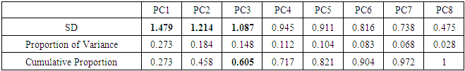
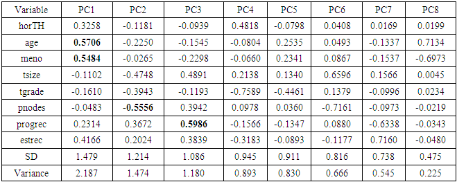
- In the proposed work, we have implemented the principal component analysis and clustering on variables on two data sets, breast cancer and ALL data sets to evaluate their performance in reducing dimension of these two data sets.For Breast cancer our findings exhibited in Fig. 1, Fig. 2, Fig.3, Fig. 4, Tables 1 and 2. we conclude that dimension of data set is reduced from eight to three when we use principal component analysis with four important variables (age, meno, pnodes, progrec). These three PCs explain about 60% of the total data variance hence here we lost about 40% of the information regarding the variance covariance structure.About the clustering on variables our findings show a reduction of the dimension from eight to five with out losing any of information. We can reduce the set of variable to may be {progress, age, meno, tgrade and pnodes} or {estrec, tsize, horTh, tgrade and pnodes}.It may be noted that the principal components failed to include the important variable (tgrade) in the reduced set and the cost is loss of 40% of information. As such clustering of variable prevails over PCA in this case.For ALL data set our findings exhibited in Fig. 5, Fig.6, Fig.7, Fig.8, Tables 3 and 4. we conclude that the dimension of data set is reduced from eleven to five with principal component analysis with two important variables (kinet and sex). These five PCs explain about 77.4% total data variance hence here we lost about 22.6% of information regarding the variance covariance structure.However, when we used clustering on variables we reduce the dimension from eleven to eight with out losing any of information. Therefore we can reduce the set of variables to either {kinet, cyton, sex, t922, CR, fusionp, citog, BTd} or {remission, t411, sex, t922, CR, fusionp, citog, molb} with out losing any information as compared to the principal component analysis which fails to reduce dimension with good level of interpretation of data.In medication of patients who have cancer, time is very important so if two variables falls in one cluster one needs two days to collect data other needs ten days therefore we select variable, which needs two days, and starting classify our patient to start medication. Therefore the main recommendations from the current investigation is to use clustering on variables for reduce dimension because it is effective and there is no loss of information and gives options to select important variables from the same cluster because they are homogenous.