ElemUche O.1, Omekara C. O.2, Nsude F. I.1
1Maths / Statistics Department, Akanu Ibiam Federal Polytechnic Unwana - Afikpo, Ebonyi State, Nigeria
2Statistics Department, Michael Okpara University of Agriculture Umudike, Abia State, Nigeria
Correspondence to: ElemUche O., Maths / Statistics Department, Akanu Ibiam Federal Polytechnic Unwana - Afikpo, Ebonyi State, Nigeria.
| Email: |  |
Copyright © 2018 The Author(s). Published by Scientific & Academic Publishing.
This work is licensed under the Creative Commons Attribution International License (CC BY).
http://creativecommons.org/licenses/by/4.0/

Abstract
This paper focused on the causality relationship test with application to monetary policy transmission channels for Nigeria in the framework of vector autoregressive (VAR) model. Data used consist of three main monetary policy transmission channels (credits, exchange rate and interest rate) and are arranged on monthly basis, starting from January 2008 to June 2016. Granger causality analysis was carried out on the data in order to assess the potential predictability of one channel(s) to the others. The result shows a unidirectional causality relationship between exchange rate channel and interest rate channel, and between credit channel and interest rate channel. This reveals that exchange rate channel and credit channel was useful in forecasting interest rate, but the converse is not true. Also, a pair-wise Granger Causality test shows non-directional causality between credit channel and exchange rate channel, which indicates that both channels cannot affect each other. Thus, exchange rate channel cannot be used to forecast credit channel, also the converse is true.
Keywords:
Granger Causality, Monetary policy, VAR
Cite this paper: ElemUche O., Omekara C. O., Nsude F. I., Application of Granger Causality Test in Forecasting Monetray Policy Transmision Channels for Nigeria, International Journal of Statistics and Applications, Vol. 8 No. 3, 2018, pp. 119-128. doi: 10.5923/j.statistics.20180803.02.
1. Introduction
Nigeria currently is faced with stagnated growth, unstable business cycles and economic fluctuation which have led to unemployment, inflation, unproductivity and balance of payment disequilibrium. Government on their part has in one way or the other introduced policies to regulate and control the economy in other to maximize the welfare of the citizens by ensuring that the resources available are efficiently allocated and used. Like any other developing country, Nigerian government adopts three types of public policies to carry out the objective of allocation of resources. These public policies include: monetary policy, fiscal policy and income policy tools. In Nigeria, government has always relied on monetary policy as a way of achieving certain economic objective in the economy such economic objectives include; employment, economic growth and development, balance of payment equilibrium and relatively stable general price level. Monetary policy refers to the combination of measures designed to regulate the value, supply and cost of money in an economy in consonance with the level of economic activities. It can be described as the art of controlling the direction and movement of monetary and credit facilities in pursuance of stable price and economic growth in the economy (CBN, 1992).The goal of monetary policy is to induce changes in aggregate expenditures, which result in changes in gross domestic product, the price level, inflation, employment, unemployment, and balance of payment equilibrium. The route between monetary policy and aggregate expenditures works through a variety of channels. The three main monetary policy transmission channels (variables) are: credit, interest rate and exchange rate channels. These channels generally reinforce each other, all moving aggregate expenditures in the same direction. Also, these channels increase aggregate expenditures with expansionary monetary policy and decrease aggregate expenditures with contractionary monetary policy (Hung, 2011).The relationship between monetary policy transmission variables and the economy (GDP) has been analyzed by many authors. For instance, Onyeiwu (2012), Owalabi and Adegbite (2014), Adefeso and Mobolaji (2010), Chukwu (2009), Micheal and Ebibai (2014), Okwo, et al., (2012). These works were based on regressing one variable on the other(s) with no recourse to causality influences/effects. Causality is the improvement of a time series variable by incorporating the information about another variable. Thus, would one time series variable improve the prediction of the other variable(s) if the information about the first is incorporated? The major issue is in the forecasting ability of the policy channels in the economy visa-vise the predicting power of one to another. Therefore, this article presents a platform on how knowledge information of one time series variable would be a precursor to predict other(s). In other words, the paper seeks to presents fundamental casual connectivity of time series variables vis-à-vis monetary policy transmission channels in an economy.
1.1. Granger Causality
A time series variable is called ‘causal’ to another if the ability to predict the second variable is improved by incorporating information about the first. The notion of causality was first proposed in (Wiener, 1956). However, at that time Wiener lack practical implementation of this idea and Granger (1969) came up with the implementation format in context of time series linear auto regressive models of stochastic processes.Granger causality is a technique for determining whether one time series is useful in forecasting another. Granger (1969) defined causality as follows:A variable Y is causal for another variable X if knowledge of the past history of Y is useful for predicting the future state of X over and above knowledge of the past history of X itself. So if the prediction of X is improved by including Y as a predictor, then Y is said to be Granger causal for X.Granger-causality test can be applied in three different types of situations:1. In a simple Granger-causality test there are two variables and their lags.2. In a multivariate Granger-causality test more than two variables are included, because it is supposed that more than one variable can influence the results.3. Granger-causality can also be tested in a VAR framework; in this case, the multivariate model is extended in order to test for the simultaneity of all included variables.Causality between two variables can be unidirectional, bidirectional (or feedback) and neither bilateral nor unilateral (i.e. independence means no Granger-causality in any direction). Granger causality testing applies only to statistically stationary time series. If the time series are non-stationary, then the time series model should be applied to temporally differenced data rather than the original data.The test procedure as described by (Granger, 1969) is stated below as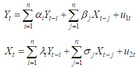 The first equation postulates that the current
  is related to its past values as well as that of
  and vice versa. Unidirectional causality from
  and
and  is indicated if the estimated coefficient on the lagged
  are statistically different from zero as a group (i.e.
  ) and the set of estimated coefficient on the lagged
  are not statistically different from zero if
  . The converse is also the case for unidirectional causality from
  to
to  . Feedback or bilateral causality exist when the sets of
  and
and  coefficients are statistically different from zero in both above regressions (Gujarati, 2009).
2. Methodology
The data used in this paper consist of three monetary policy transmission channels, namely Interest rate channel (IR), Exchange rate channel (ER) and Credit channel (CR). The data are monthly and were sourced from the Central Bank of Nigeria Statistical bulletin. The data has 102 observations, starting, January 2008 to June 2016.The data sourced were analyzed to determine the causality between CR and ER, CR and INT, and finally ER and INT. Before analyzing the causal relationship between the monetary transmission channels, data were transformed to natural logarithms, and then examined for possible existence of unit roots in the data to ensure that the model constructed later is stationary in terms of the variables used. If a time series has a unit root, then the first difference of the series which is stationary should be used. The stationarity of each series is investigated by employing Augmented Dickey-Fuller unit root test. We further proceed with the VAR lag order selection criteria to choose the best lag length for the VAR time series model to examine the Granger causality and we perform the pair wise Granger Causality test for all the series. To carry out the analysis of the data, we used the statistical package, E-views® version 9 which is used mainly for econometric analysis.
2.1. Modeling/ Theoretical Approach
1. Determine if there exists a unit root or stationarity.2. Obtain the VAR lag order selection 3. Perform the pair Granger causality test.
2.2. Stationarity
Walter (2004) defined Stationarity as follows:A time series yt is covariance (or weakly) stationary if, and only if, its mean and variance are both finite and independent of time, and the auto-covariance does not grow over time, for all t and t-s. Non-stationarity exists when the variance is time dependent and goes to infinity as time approaches to infinity. A time series which is not stationary with respect to the mean can be made stationary by differencing. Differencing is a popular and effective method of removing a stochastic trend from a series.
2.2.1. Testing of Stationarity
If a time series has a unit root, the series is said to be non-stationary. Tests which can be used to check the stationarity are:1. Partial autocorrelation function and Ljung and Box statistics.2. Unit root tests - a test designed to determine whether a time series is stable around its level (trend stationary) or stable around the differences in its levels (difference-stationary).To check the stationarity and if there is presence of unit root in the series, the most famous of the unit root tests are the ones derived by Dickey and Fuller and described in Fuller (1976), also Augmented Dickey-Fuller (ADF) or Said-Dickey test has been mostly used.
2.3. Dickey-Fuller (DF) Test
Dickey and Fuller (DF) considered the estimation of the parameter α from the models:1. A simple AR (1) model is: 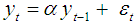 2.
2.  3.
3.  It is assumed that y0 = 0 and
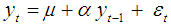
  ~ independent identically distributed, i.i.d (0, σ2)The hypotheses are: H0: α = 1 vs. H1: |α| <1Alternative three versions of the Dickey-Fuller test of the parameter α from the models:1. Pure random walk model.
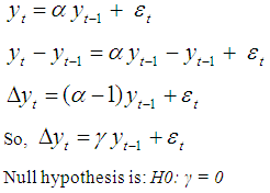 2. Drift + random walk.
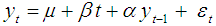
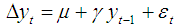 Null hypothesis is: H0: μ = 0; γ = 03. Drift + linear time trend.
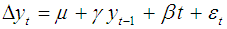 Null hypothesis is: H0: β = 0; γ = 0Where, μ is a drift or constant term, βt is a time trend, and
  is the first-order difference of the series yt.
2.4. Augmented Dickey-Fuller (ADF) or Said-Dickey Test
Augmented Dickey-Fuller test is an augmented version of the Dickey-Fuller test to accommodate some forms of serial correlation and used for a larger and more complicated set of time series models. If there is higher order correlation then ADF test is used but DF is used for AR (1) process. The testing procedure for the ADF test is the same as for the Dickey-Fuller test but we consider the AR (p) equation: 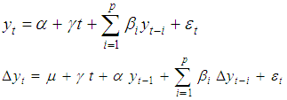 Each version of the test has its own critical value which depends on the size of the sample. In each case, the null hypothesis is that there is a unit root, γ = 0.
2.5. Vector Auto-regression (VAR)
Vector Auto-regression (VAR) is an econometric model which has been used primarily in macroeconomics to capture the relationship and independencies between important economic variables. They do not rely heavily on economic theory except for selecting variables to be included in the VARs. The VAR can be considered as a means of conducting causality tests, or more specifically Granger causality tests. VAR can be used to test the Causality as; Granger-Causality requires that lagged values of variable ‘X’ are related to subsequent values in variable ‘Y’, keeping constant the lagged values of variable ‘Y’ and any other explanatory variables. In connection with Granger causality, VAR model provides a natural framework to test the Granger causality between each set of variables. VAR model estimates and describe the relationships and dynamics of a set of endogenous variables.For a set of ‘n’ time series variables , a VAR model of order p (VAR(p)) can be written as:
  Where,p = the number of lags to be considered in the system.n = the number of variables to be considered in the system.Yt is an (n×1) vector containing each of the ‘n’ variables included in the VAR.A0 is an (n×1) vector of intercept terms.Ai is an (n×n) matrix of coefficients.εt is an (n×1) vector of error terms.
2.6. Determination of Lag-Length for VAR Model
A critical element in the specification of VAR models is the determination of the lag length of the VAR. Various lag length selection criteria are defined by different authors like, Akaike (1969) final prediction error (FPE), Akaike Information Criterion (AIC) suggested by Akaike (1974), Schwarz Criterion (SC) (1978) and Hannan-Quinn Information Criterion (HQ) (1979).
2.7. Information Criteria
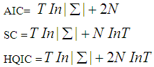 Where,
  = determinant of the variance/covariance matrix of the residuals. N = total number of parameters estimated in all equations. T = number of usable observations.
3. Results of Graphical Presentation and Application
This section consists of graphical presentation of data and applications of unit root test, VAR lag order selection criteria and pair-wise Granger Causality.The research starts by showing the graphs of the raw data, which comprises the series CR, ER and INT in order to know how they behave in their natural state. The (Fig. 1, Fig. 2 and Fig. 3) are shown below.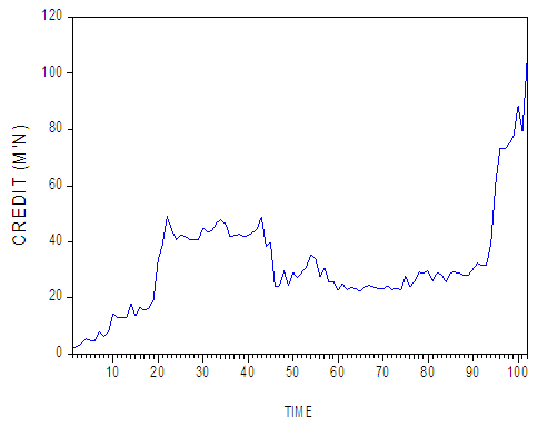 | Figure 1. (Graph of CR) |
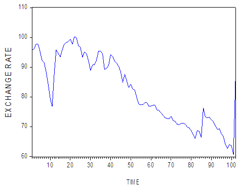 | Figure 2. (Graph of EX) |
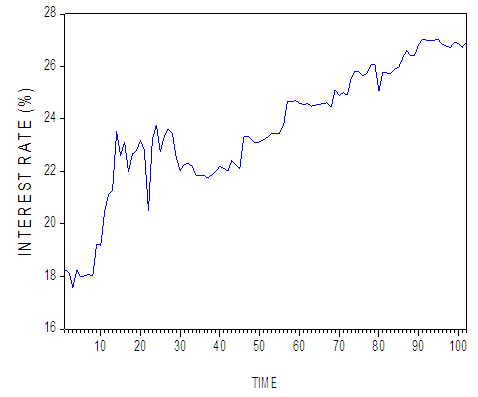 | Figure 3. (Graph of INT) |
From the above three figures, the impression is that the series are not stationary.Our next step is to make the series linear. We take the logarithms of the original series: CR, EX, and INT and produce their graphs. To conclude that the series are stationary or not, we also produce the correlograms of the three logarithmic series: LNCR, LNEX, and LNINT (Fig. 4, Fig. 5 and Fig. 6).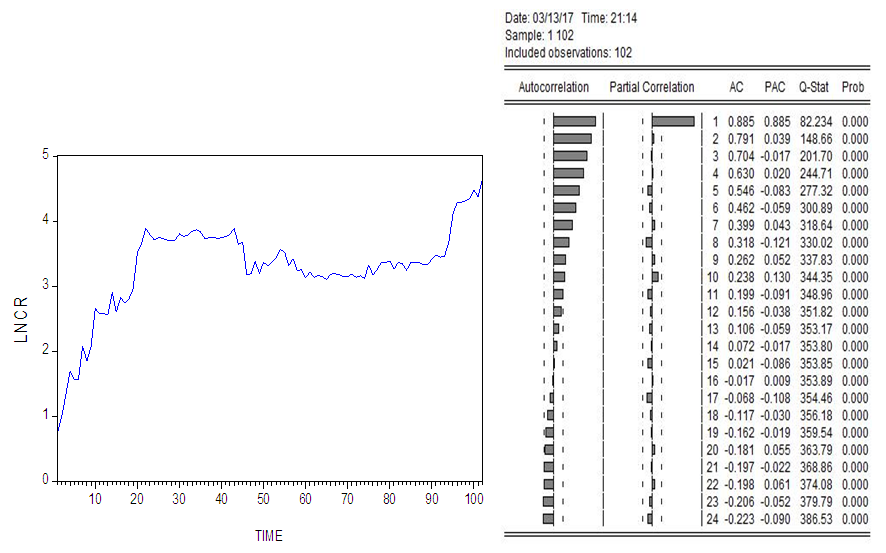 | Figure 4. (Graph and Correlogram of LNCR) |
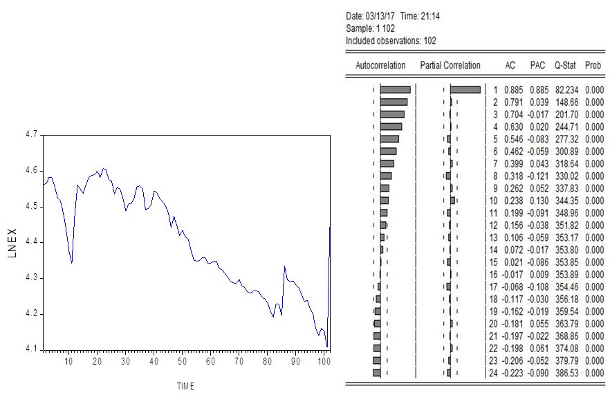 | Figure 5. (Graph and Correlogram of LNEX) |
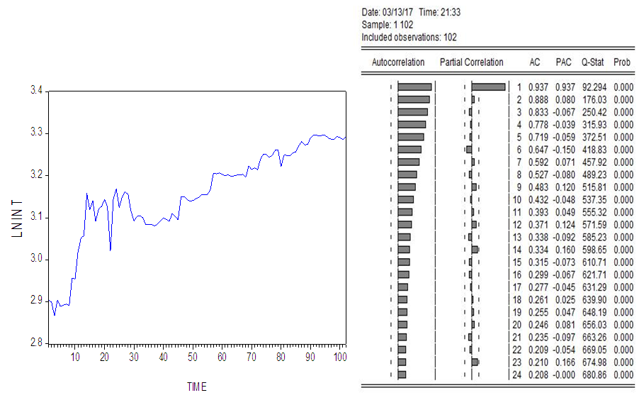 | Figure 6. (Graph and Correlogram of LNINT) |
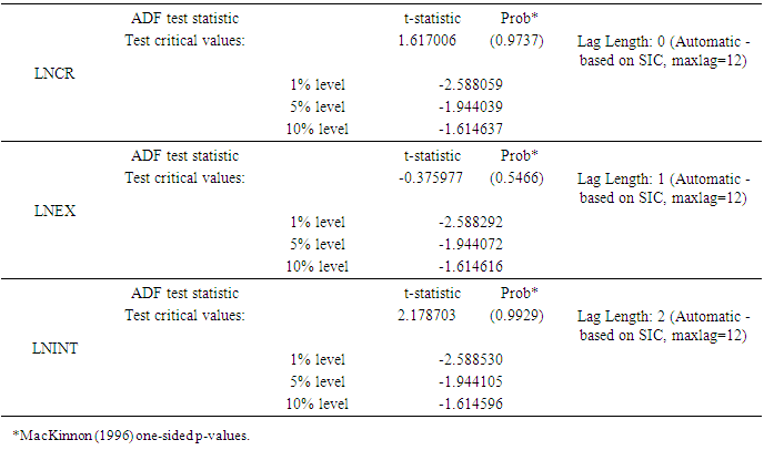
From the above graphs, we conclude that all the three series are not stationary also the above correlograms do not show stationarity. It is clear from correlograms that the non-decaying behavior of the sample Autocorrelation Function (ACF) is due to lack of stationarity because ACFs are suffered from linear decline but the Partial Autocorrelation Function (PACFs) decaying very quickly and there is only one significant spike of PACFs.To make the above conclusion more confirm, we perform a unit root test (Augmented Dickey-Fuller) to observe whether the series are stationary or not.Table 1. (Augmented Dickey-Fuller ADF Test on LNCR, LNEX, LNINT) Null hypotheses: LNCR, LNEX, LNINT has a unit root
 |
| |
|
Above table is the summary of results of Augmented Dickey-Fuller test. According to (Table.1), we conclude that there is presence of unit root according to the P-values of all the three series as the P-values are insignificant. Since the values of computed ADF test-statistic of the three series are greater than the critical values at 1%, 5% and 10% levels of significance, respectively with different lag lengths (based on Schwarz Information Criterion). So, the null hypotheses cannot be rejected that means all the three series have a unit root.Hence, from the unit root test, we conclude that the three series are not stationary, so we make these three non-stationary series, stationary by taking first difference as: DLNCR, DLNEX and DLNINT. Below graphs and correlograms clearly shows the first difference of the series.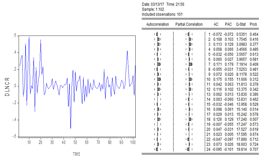 | Figure 7. (Graph and correlogram of DLNCR) |
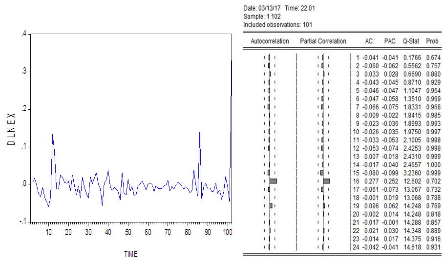 | Figure 8. (Graph and correlogram of DLNEX) |
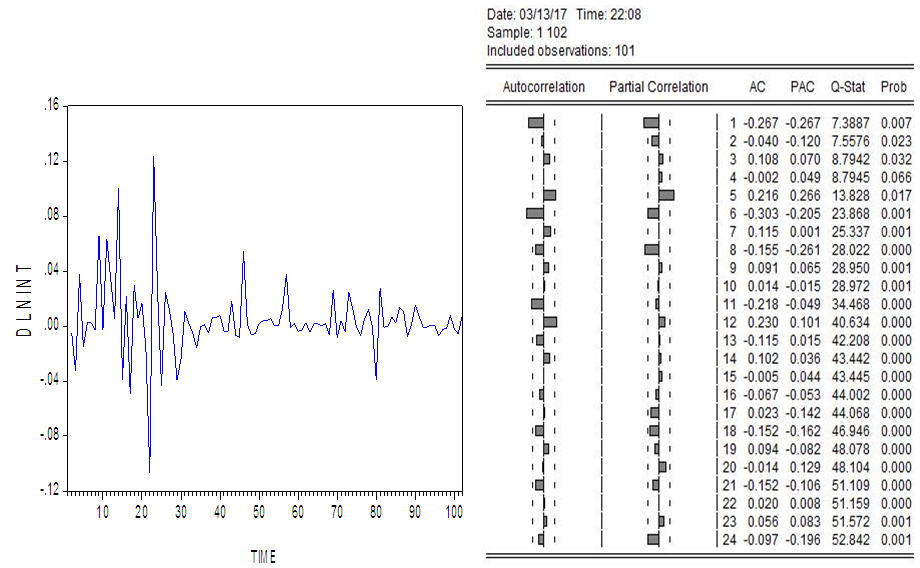 | Figure 9. (Graph and Correlogram of DLNINT) |
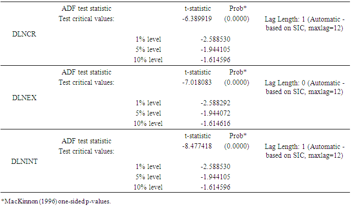
A first difference of all the three series looks stationary and correlograms also verifies the same as we see that ACFs tend to zero rather quickly. We apply unit root test with Augmented Dickey-Fuller after taking the first difference to check whether the series are now stationary or not.Table 2. (Augmented Dickey-Fuller ADF Test on DLNCR, DLNEX, DLNINT) Null hypotheses: DLNCR, DLNEX, DLNINT has a unit root
 |
| |
|
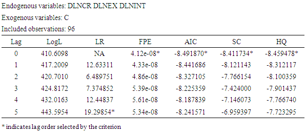
According to the summary results of Augmented Dickey-Fuller test above (Table. 2), we conclude that there is absence of unit root according to the P-values of all the three series as the P-values are significant. The values of computed ADF test-statistic of the three series are smaller than the critical values at 1%, 5%, and 10% levels of significance, respectively with different lag lengths (based on Schwarz Information Criterion). Therefore, we reject the null hypotheses that all the three series do not have a unit root. We conclude that all the three series are stationary according to the results of Augmented Dickey-Fuller (Table. 2).Since the three series are stationary, we precede with the lag order selection criteria for testing the Granger Causality. Lag length selection criteria was determined using the VAR model. We select the best lag length for the VAR time series model on which Granger causality is based (Table. 3).Table 3. VAR lag order selection Criteria
 |
| |
|
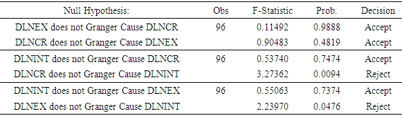
According to the results of VAR lag order selection criteria (Table. 3), we decide to use lag length 5 for the Granger Causality test. This is due to the fact that FPE, Akaike, Schwarz and Hannan-Quinn choose 0 lags but LR chooses 5 lags. We use the LR test [sequential modified LR test statistic (each test at 5% level)] as a primary determinant of how many lags to be include.With continuation of analysis, we proceed to perform the pair-wise Granger Causality test for all the series DLNCR, DLNEX and DLNINT (Table. 4) by using the above selected lag length 5.Table 4. Pair-wise Granger Causality Tests
 |
| |
|
Pair-wise comparison of series, DLNCR VS DLNEXAccording to the results of (Table 4), the P-value (0.9888) is not significant so, we accept the null hypothesis and we conclude that DLNEX does not Granger Cause DLNCR. The P-value (0.4819) is also not significant so, we accept the null hypothesis and we conclude that DLNCR does not Granger cause DLNEX. So, DLNEX does not affect DLNCR and the converse is also true, it means that there is no Granger Causality between the series, running from DLNEX to DLNCR and the other way. Hence, the Granger Causality is non-directional between the series.Pair-wise comparison of the series, DLNCR VS DLNINTAccording to (Table 4), the P-value (0.7474) is not significant so, we accept the null hypothesis and we conclude that DLNINT does not Granger cause DLNCR. But the converse is not true as P-value (0.0094) is significant. So, we reject the null hypothesis and we conclude that DLNCR Granger Cause DLNINT. So, DLNCR affects DLNINT but the converse is not true, it means the Granger Causality is unidirectional between the series, DLNCR and DLNINT, running from DLNCR to DLNINT and not the other way.Pair-wise comparison of series, DLNEX VS DLNINTAccording to (Table 4), the P-value (0.7374) is insignificant so, we cannot reject the null hypothesis and we conclude that DLNINT does not Granger Cause DLNEX. The P-value (0.0476) is significant so, we reject the null hypothesis and we conclude that DLNEX Granger Cause DLNINT. So, DLNEX affects DLNINT, but the converse is not true, it means the Granger Causality is unidirectional between the series.
4. Summary and Conclusions
The main objective of this paper is to analyze the causality relationship with application to credit channel CR, exchange rates channel EX and interest rate channel IR of monetary policy transmission channels. We perform unit root test, VAR lag order selection criteria and pair-wise Granger Causality test to establish the causality which exists between the three monetary policy transmission channels of our study.According to the results of this research with original data, we found that the three series have a unit root which means all the series do not show stationarity. After taking first difference of the series, the results of unit root test show stationarity at the levels of significance: 1%, 5% and 10% with different lag lengths.According to the results of pair-wise Granger Causality tests, we observed non-directional causality relationship between CR and EX, which means that the past history of both series cannot predict their future values. Thus, we conclude that EX cannot be used to forecast CR, also the converse is true.Also, we observed unidirectional causality running from CR to INT which means that the past history of CR is useful to forecast the future values of INT, but the converse is not true.Finally, we observed another unidirectional causality running from EX to INT which shows that EX is useful to forecast INT, but the converse is not true.Furthermore, according to the results of Granger-Causality of our research, we observe that the casual relationship which exists between CR, EX and INT adjust to reflect changes in the monetary policy transmission channels of Nigeria. The leading role of the Credit channel and Exchange rate channel affecting Interest rate channel is clearly visible in the causality relationship tests.
References
| [1] | Adefeso, H. & Mobolaji, H. (2010). The fiscal–monetary policy and economic growth in Nigeria: Further Empirical Evidence. Pakistan Journal of Social Sciences, 7 (2), 137-142. |
| [2] | Akaike, H. (1969). Fitting autoregressive models for prediction. Annals of the Institute of Statistical Mathematics, (21), 243-247. |
| [3] | Akaike, H. (1974). A new look at the statistical model identification. IEEE Transactions on Automatic Control, (19), 716-723. |
| [4] | CBN (2008). Central Bank of Nigeria (CBN), Monetary Policy Department Series 1, 2008.CBN/MPD/Series/01/2008. www.cbn. |
| [5] | CBN (2016). Statistical Bulletin; 2016. |
| [6] | Enders W. (2004). Applied Econometric Time Series. 2nd Edition, New York: Wiley. |
| [7] | Granger, C. W. J. (1969). Investigating Causal Relationship by Econometric Model and Cross-spectral Methods. Econometrica, (37), 424-438. |
| [8] | Granger, C. W. J. (1981). Some properties of time series data and their use in econometric model specification. Journal of Econometrics, (16), 121-130. |
| [9] | Gujarati, D. N. & Porter, D.C. (2009). Basic econometrics. Fifth edition, New York, McGraw-Hill/Irwin. |
| [10] | Hannan, E. J. & B. G. Quinn (1979). The determination of the order of an auto-regression. Journal of the Royal Statistical Society, Series B 41, 190-195. |
| [11] | Hung, L. V. (2011), AVector Autoregression Analysis of Monetary Transmission Mechanism in Vietnam, National Graduate Institute of Policy Studies (GRIPS). |
| [12] | Michael, B. & Ebibai, T. S. (2014). Monetary policy and economic growth in Nigeria (1980-2011). Asia Economic and Financial Review, 4(1). 20-32. |
| [13] | Okwo, I. M. Eze, F. & Nwoha, C. (2012). Evaluation of monetary policy outcomes and its effect on price stability in Nigeria. Research Journal Finance and Accounting, 3 (11), 37-47. |
| [14] | Onyeiwu, C. (2012). Monetary policy and economic growth of Nigeria. Journal of Economic and Sustainable Development. 3(7). 62-70. |
| [15] | Owalabi, A. U. & Adegbite, T. A. (2014). Impact of monetary policy on industrial growth in Nigeria. International Journal of Academic Research in Business and Social Sciences, 4 (1), 18-31. |
| [16] | Schwarz, G. (1978). Estimating the dimension of a model. The Annals of Statistics, (5), 461-464. |
| [17] | Wiener, N. (1956). The theory of prediction. In: Beckenbach, E. (Ed.), Modern Mathematics for Engineers. New York, McGraw-Hill. |

 Abstract
 Reference
 Full-Text PDF
 Full-text HTML