Omosigho Donatus Osaretin, Audu Adejumoke Tolulope, Fadayomi Akinwunmi Festus
Department of Mathematics and Statistics, Federal School of Statistics, Ibadan, Nigeria
Correspondence to: Omosigho Donatus Osaretin, Department of Mathematics and Statistics, Federal School of Statistics, Ibadan, Nigeria.
| Email: |  |
Copyright © 2018 The Author(s). Published by Scientific & Academic Publishing.
This work is licensed under the Creative Commons Attribution International License (CC BY).
http://creativecommons.org/licenses/by/4.0/

Abstract
In this paper, we introduce a new distribution called kumaraswamy transmuted inverted Weibull (KTIW) distribution. The new distribution was used in analyzing bathtub failure rates lifetime data. We consider the standard transmuted inverted Weibull distribution (KTIW) distribution that generalizes the standard inverted Weibull distribution (IWD), the new distribution has four shape parameters. The moments, median, reliability function, Quantile function, hazard function, maximum likelihood estimators and fisher information matrix obtained. A real data set was analyzed and it was observed that the (KTIW) distribution can provide a better fitting than (IWD) distribution.
Keywords:
Moments, Bathtub failure rate, Reliability function, Quantile function
Cite this paper: Omosigho Donatus Osaretin, Audu Adejumoke Tolulope, Fadayomi Akinwunmi Festus, On Statistical Properties of the Kumaraswamy Transmuted Inverted Weibull Distribution, International Journal of Statistics and Applications, Vol. 8 No. 2, 2018, pp. 103-110. doi: 10.5923/j.statistics.20180802.09.
1. Introduction
The inverted Weibull distribution is one of the most popular probability distribution to analyze the life time data with some monotone failure rates. Ref. [1] studied the properties of the inverted Weibull distribution and its application to failure data. Ref. [2] introduced the exponentiated Weibull distribution as generalization of the standard Weibull distribution and applied the new distribution as a suitable model to the bus-motor failure time data. Ref. [3] reviewed the exponentiated Weibull distribution with new measures. Many Kumaraswamy distribution have been proposed in the literature: kumaraswamy Gumbel distribution due to Ref. [4], the Kumaraswamy Birbaum-saunders distribution due to Ref. [5], the kumaraswamy log-logistics distribution due to Ref. [6], the kumaraswamy generalized gamma distribution due to Ref. [7], the kumaraswamy Burr xii distribution due to Ref. [8], the kumaraswamy Weibull was due Ref. [9]. In this article we use the kumaraswamy transmuted-G family of distribution by Ahmed Z. Afify et. al (2016) which the cumulative density function (cdf) is given by | (1) |
The probability density function (PDF) is given by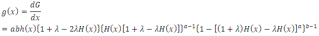 | (2) |
Where  and
and  is the pdf and the cdf of the base line distribution respectively.
2. Kumaraswamy Transmuted Inverted Weibull Distribution (KTIW) Distribution
We say that the random variable X has a standard inverted Weibull distribution (IWD) if its distribution function takes the following form: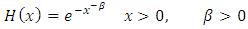 | (3) |
The pdf of Inverted Weibull distribution is given by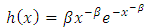 | (4) |
Now using (3) and (1) we have the cdf of a (KTIW) distribution given by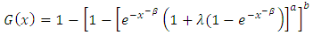 | (5) |
Where  is simply the transmutation parameter of the distribution function of the standard inverted Weibull distribution (IWD). Here
  and
and  are the shape parameters. Therefore, the probability density function is given as
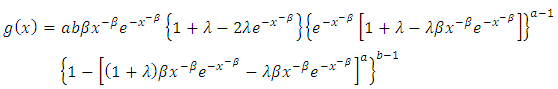 | (6) |
Note that for  we have the pdf of a standard inverted Weibull distribution. Fig. 1 and fig. 2 illustrate some of the possible shapes of the density function of (KTIW) distribution for selected parameters.
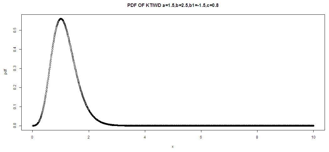 | Figure 1. The graph of the pdf of KTIW distribution |
The above graph shows that the KTIW unimodal and right skewed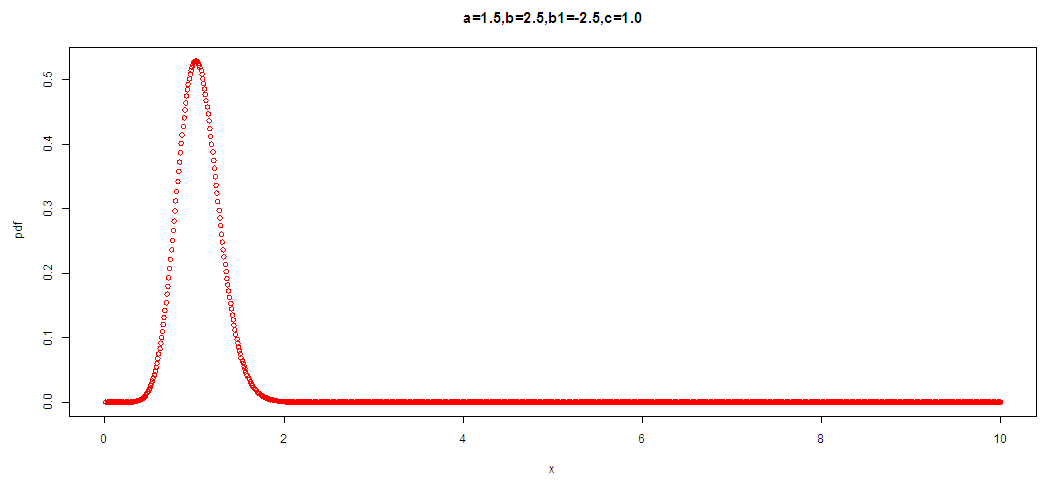 | Figure 2. From the pdf graph drawn above we can deduce that the KTIW distribution is unimodal and right tailed |
3. Mixture Representation of the Function
Consider the power series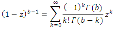 | (7) |
Which holds for  real none—integer.Applying power series in (7) to equation (6) we obtain
 | (8) |
Where | (9) |
4. Moments, Mean, Variance, Median
In this section we shall present the moments and qunatiles for the (KTIWD). The  order moments of (KTIW) distribution can be obtained as follows for a random variable X,
  | (10) |
Putting eq. (6) in eq. (10), we have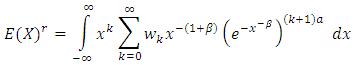 | (11) |
This gives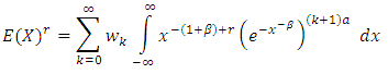 | (12) |
If we let 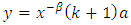 in eq. (12) Finally we have
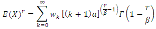 | (13) |
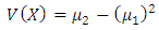
It should be noted that  .The mean of (KTIW) distribution is the first moment about the origin
  which corresponds to eq. (13).And the variance of (KTIW) distribution can be obtained using the relation.The first moment and second can be obtained by taking the value of
 | (14) |
For  , then
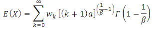 | (15) |
And the second moment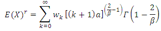 | (16) |
Inserting eq. (15) and eq. (16) in eq. (17) we have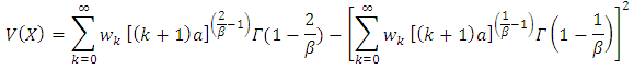 | (17) |
5. Quantile Function
The quantile function for the (KTIW) distribution by inverting the cdf in equation (5) given as,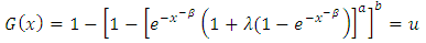 | (18) |
Then we have,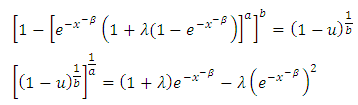 | (19) |
If we let  in equation (19)
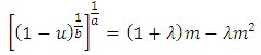 | (20) |
Solving equation (20) using quadratic formula, then we have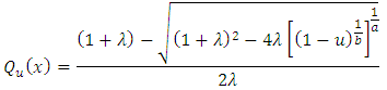 | (21) |
The lower quartile, median and the upper quartile of the (KTIW) distribution can be obtained by letting  and
and  respectively in eq. (21).
6. Reliability Analysis
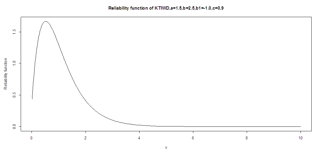
The survival function, also known as the reliability function in engineering, is the characteristic of an explanatory variable that maps a set of events, usually associated with mortality or failure of some certain mechanical wearing system with time. It is the conditional probability that the system will survive beyond a specified time. The reliability function define as, 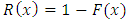 , for (KTIW) distribution is given by:
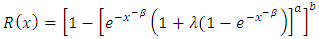 | (22) |
The other characteristic of interest of a random variable is the hazard rate function also known as instantaneous failure rate defined by | (23) |
Is an important quantity characterizing life phenomenon. It can be loosely interpreted as the conditional probability of failure, given it has survived to the time t: The hazard rate function for a (KTIW) distribution is given by | (24) |
The figure 3 and 4 clearly indicates the flexibility of KTIW distribution as it was constant and increasing in fig. 3 and increasing, decreasing and constant in fig. 4.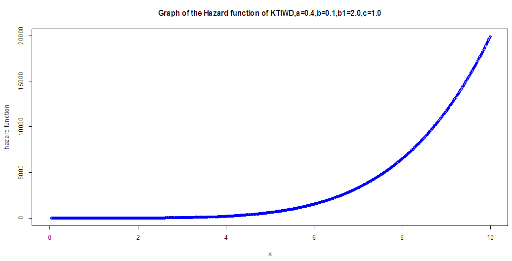 | Figure 3. The graph of hazard rate function for KTIW distribution |
 | Figure 4. The graph of hazard rate function for KTIW distribution |
7. Moment Generating Function of (KTIW) Distribution
The moment generating function of a random variable x is defined by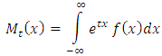 | (25) |
The above expression can further be simplify as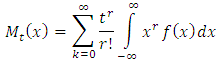 | (26) |
Since, | (27) |
Inserting eq. (13) in eq. (26) we have | (28) |
The above expression is the moment generating function of (KTIW) distribution.
8. Entropy
The entropy of a random variable X with probability density  is a measure of variation of the uncertainty. A large value of entropy indicates the greater uncertainty in the data. The Renyi, A. (1961) introduced the Renyi entropy defined as
 | (29) |
Where  and
and  . The integral in
  of the
  distribution can be define as
 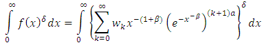 | (30) |
This can be simplify as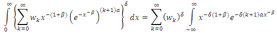 | (31) |
By letting, 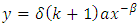 in the above equation, we have
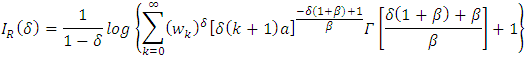 | (32) |
9. Maximum Likelihood Estimators and Fisher Information Matrix
If  is a random sample from kumaraswamy transmuted inverted Weibull distribution given by (6), then the Likelihood function (L) becomes:
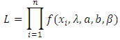 | (33) |
By substituting from equation (6) into Equation (33), we get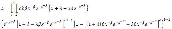 Then the log – likelihood function becomes
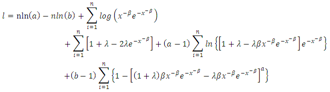 | (34) |
And the score vector is given as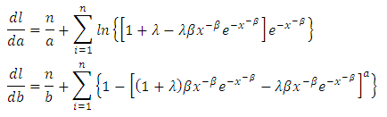 | (35) |
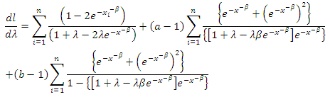 | (36) |
The maximum likelihood estimator 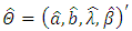 of
of 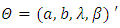 is obtained by setting the score vector to zero and solving the nonlinear system of equations. It is usually more convenient to use nonlinear optimization algorithms such as quasi- Newton algorithm to numerically maximize the log-likelihood function given in ().
10. Application
In this section, we use two real data sets to show that the KTIW distribution can be a better model than one based on the inverted Weibull (IW) distribution and the exponentiated inverted Weibull (ETIW) distribution. In the application, we consider a data set of the tensile strength of 100 observations of carbon fibers. These data are: 3.7, 2.74, 2.73, 2.5, 3.6, 3.11, 3.27, 2.87, 1.47, 3.11, 4.42, 2.41, 3.19, 3.22, 1.69, 3.28, 3.09, 1.87, 3.15, 4.9, 3.75, 2.43, 2.95, 2.97, 3.39, 2.96, 2.53, 2.67, 2.93, 3.22, 3.39, 2.81, 4.2, 3.33, 2.55, 3.31, 3.31, 2.85, 2.56, 3.56, 3.15, 2.35, 2.55, 2.59, 2.38, 2.81, 2.77, 2.17, 2.83, 1.92, 1.41, 3.68, 2.97, 1.36, 0.98, 2.76, 4.91, 3.68, 1.84, 1.59, 3.19, 1.57, 0.81, 5.56, 1.73, 1.59, 2, 1.22, 1.12, 1.71, 2.17, 1.17, 5.08, 2.48, 1.18, 3.51, 2.17, 1.69, 1.25, 4.38, 1.84, 0.39, 3.68, 2.48, 0.85, 1.61, 2.79, 4.7, 2.03, 1.8, 1.57, 1.08, 2.03, 1.61, 2.12, 1.89, 2.88, 2.82, 2.05, 3.65. Table 1 gives the exploratory data analysis of the data considered, Table 2 gives the maximum likelihood estimates of the parameters with their standard error in parenthesis and Table 3 gives the criteria for comparison. Fig. 5 represents the empirical density and the cumulative density of the data considered. Table 1. Descriptive Statistics on Breaking stress of Carbon fibres
 |
| |
|
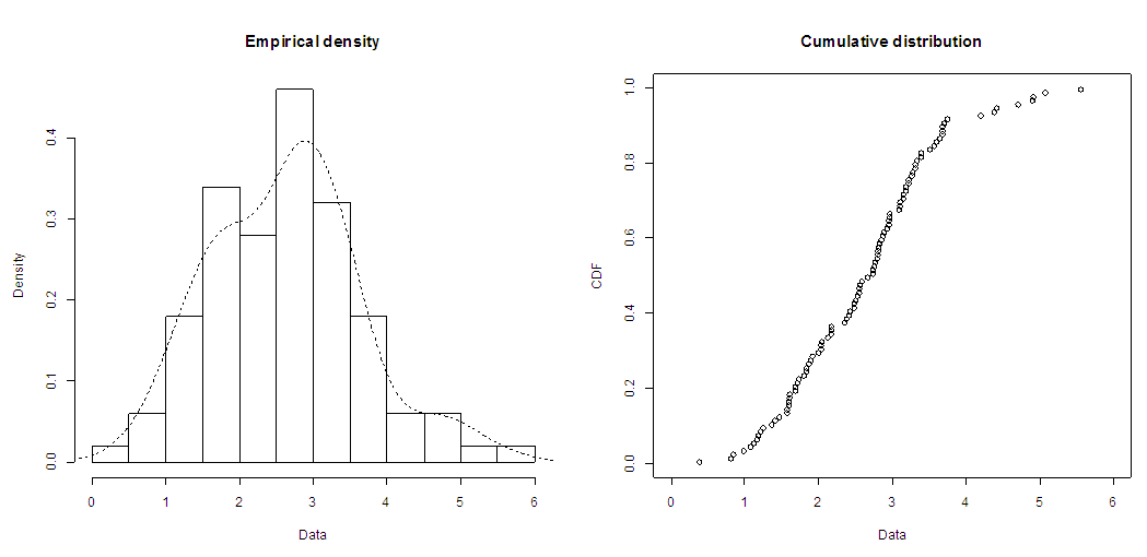 | Figure 5. The graph of the Empirical density and the cumulative distribution function of the carbon data |
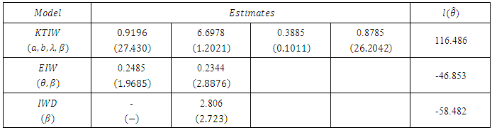
Table 2. Estimated parameters of the KTIW, EIW and IWD distribution
 |
| |
|
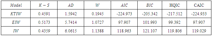
Table 3. Measures of Goodness of Fit
 |
| |
|
We employ the statistical tools for model comparison such as Kolmogorov-Smirnov (K-S) statistics, Anderson Darling statistic (AD), crammer von misses statistic (W), Akaike information criterion (AIC), Consistent Akaike information criterion (CAIC), Hannan Quinine information criterion (HQIC) and Bayesian information criterion o choose the best possible model for the data sets among the competitive models. The selection criterion is that the lowest AIC, CAIC, BIC and HQIC correspond to the best fit model.
11. Conclusions
Among the models considered the best model is the Kumaraswamy transmuted inverted Weibull distribution for the data sets considered.
References
| [1] | A. Flair, H. Elsalloukh, E. Mendi and M. Milanova. The exponentiated inverted Weibull Distribution, Appl. Math. Inf. Sci. 6, No. 2, 167-171 (2012). |
| [2] | G.S. Mudholka, D.K. Srivastava and M. Freimer, The exponentiated Weibull family: a real analysis of the bus motor failure data. |
| [3] | G. S. Mudholkar and A. D. Hutson, Exponentiated Weibull family: some properties and flood data application, Commun. Statistical Theory and Method. 25, 3050-3083 (1996). |
| [4] | Gauss M Cordeiro, Saraless Nadarajah and Edwin M M. The Kumaraswamy Gumbel distribution. Statistical methods and applications, 21(2): 139-168, 2012. |
| [5] | Helton Saulo, Jeremias Leao and Marcelo Bourgingnon. The kumaraswamy Birnbaum-Sanders distribution Journal of Statistical Theory and practice. 6(4): 745-759, 2012. |
| [6] | Tiago viana Florde Santana, Edwin M M Ortega, Gauss M Cordeiro and Giovana O Silva. The kumaraswamy lo-logistic distribution. Journal os statistical theory and application. 11(3): 265-291, 2012. |
| [7] | Marcelino A.R de Pascoa, Edwin M M Ortega and Gauss M Cordeiro. The kumaraswamy Generalized Gamma distribution with application in survival analysis. Statistical methodology, 8(5): 411-433, 2011. |
| [8] | Gauss M Cordeiro, Edwin M M Orterga and Saraless Nadarajah. The kumaraswamy Weibull distribution with application to failure data. Journal of franklin Institute. 347 (8): 1399-1429, 2010. |
| [9] | Renyil, A. L. (1961). On Measure on Entropy and Information. In fourth Berkeley symposium on mathematical statistics and probability. (Vol. 1, pp. 547-561). |
| [10] | R.C. Gupta and R.D. Gupta (2007), "Proportional reversed hazard model and its applications", Journal of Statistical Planning and Inference, vol. 137, no. 11, 3525 - 3536. |
| [11] | M. S. Khan, G. R. Pasha and A. H. Pasha, Theoretical analysis of inverse Weibull distribution, WSEAS Transactions on Mathematics, 7, 2 (2008). |

 Abstract
 Reference
 Full-Text PDF
 Full-text HTML