-
Paper Information
- Paper Submission
-
Journal Information
- About This Journal
- Editorial Board
- Current Issue
- Archive
- Author Guidelines
- Contact Us
International Journal of Statistics and Applications
p-ISSN: 2168-5193 e-ISSN: 2168-5215
2018; 8(2): 88-102
doi:10.5923/j.statistics.20180802.08

Impact of Interactions between Collinearity, Leverage Points and Outliers on Ridge, Robust, and Ridge-type Robust Estimators
 Abstract
 Reference
 Full-Text PDF
 Full-text HTML
O. Ufuk Ekiz
Department of Statistics, Faculty of Science, Gazi University, Ankara, Turkey
Correspondence to: O. Ufuk Ekiz, Department of Statistics, Faculty of Science, Gazi University, Ankara, Turkey.
| Email: |  |
Copyright © 2018 The Author(s). Published by Scientific & Academic Publishing.
This work is licensed under the Creative Commons Attribution International License (CC BY).
http://creativecommons.org/licenses/by/4.0/

This study proposes a framework to compare performances of various ridge, robust and ridge-type robust estimators when a data set is contaminated by collinearity, collinearity-influential observations, as well as outliers. This is achieved by first generating fifteen different synthetic data sets with known level of contamination. These data sets are then used to evaluate performances of twelve different estimators based on the Monte-Carlo estimates of total mean square, total variance and total bias. It has shown that these results can be used as lookup tables to select the best estimator for various cases of contamination. The results reveal that the interactions between leverage points and collinearity can be misleading for estimation selection problem. It is also shown that the notion of directionality of outliers and the strength of collinearity can also drastically impact estimator performance. Finally, an example application is presented to validate the results.
Keywords: Collinearity-influential, Leverage, Outliers, Ridge, Robust, Ridge-type robust
Cite this paper: O. Ufuk Ekiz, Impact of Interactions between Collinearity, Leverage Points and Outliers on Ridge, Robust, and Ridge-type Robust Estimators, International Journal of Statistics and Applications, Vol. 8 No. 2, 2018, pp. 88-102. doi: 10.5923/j.statistics.20180802.08.
Article Outline
1. Introduction
- There is a growing interest in the literature for understanding the performance of ridge, robust, and ridge-type robust estimators that are less prone to the contaminations caused by outliers and collinearity in data [1-7]. However, the degree to which these contaminations effect estimator performance is not yet well understood. Hence, for practical applications this lack of insight makes it challenging to decide the best and the most efficient estimator. Another challenge is to construct proper platforms for comparing and validating estimator performances when data is subject to various levels of contaminations due to collinearity, outliers, leverage points and their interactions. In the rest of the study, the term contamination will be used to describe the negative effects of various levels of collinearity, type of outliers, leverage points and their interactions on the estimation performance. This study proposes a framework to address some of these challenges.To begin our discussion, we consider the linear regression model [8],
 | (1) |
 is an
is an  full rank design matrix, n is the sample size, and p is the number of explanatory variables. In Equation (1),
  is an
is an  error vector that satisfies the expected value
  and covariance
  where I is the
  identity matrix. Moreover,
  is the
  unknown parameter vector, and
  is the variance. In this setup, it is well known that ordinary least squares (OLS)
 | (2) |
 is the transpose of matrix X. However, it is also known that collinearity in data introduces sign switches for the OLS estimator and inflates its variance [1,3,4]. There is a vast amount of work in literature [4,9,10,11] that have proposed and studied ridge regression which is one of the most commonly used methods to overcome the challenges introduced by collinearity [3]. Furthermore, these studies have revealed that presence of high-leverage points (observations) in data is also critical since they can drastically change the effect of collinearity in estimation.Not only collinearity but outliers may also effect the performance of OLS and ridge estimators. In their studies [7,12,13], authors have proposed various robust estimators that target to eliminate the impact of outliers in estimation. Properties of these estimators vary depending upon the type of outliers present in the data; i.e. if the observations are classified as outliers based on their X (Type 1) or Y (Type 2) distances then estimator performance may vary when data contains only Type 1, only Type 2 or both Type 1 and Type 2 outliers. Finally, ridge-type and Liu-type robust estimators have been proposed in studies [1,2,5,6,14] in order to overcome the effects caused by both collinearity and outliers. However, the interactions between collinearity, outliers and leverage points are not yet well understood and it is not trivial to conclude which estimator performs better when data is subject to various levels of contamination.In [15] and [16], the impact of outliers on the performance of various robust estimators when the sample size is small is studied. In this study, the details of a simulation study in which the synthetic data sets are generated so as to involve predefined levels of contamination caused by outliers, collinearity and leverage points are presented. Then, performances of a subset of well-known ridge, robust and ridge-type robust estimators are investigated. This is achieved by first classifying collinearity-influential observations (high-leverage points) in data into three subgroups based on their type of influence-leverage-masking collinearity, leverage-inducing collinearity, and leverage-intensifying collinearity (similar classifications were presented in studies [17] and [18]).We simulate and present example data sets in Figure 1 to illustrate masking, inducing and intensifying effects of high-leverage observations on the estimate of variance inflation factor
  , where
  is the estimate of maximum determination coefficient computed for all explanatory variables such that
  is the maximum value of the diagonal elements of inverse sample correlation matrix of the explanatory variables [19,20]. Moreover,
  and
and  are the estimates of
  and
and  . Thus, when
  is the maximum determination coefficient among the explanatory variables
  . In the figure
  is an observation, where
  . Let us consider the observation
  (shown in blue) in Figure 1a. It is obvious that even if we exclude
  there exists collinearity between the rest of the observations. However, it is also clear that including
  in the computations will intensify the strength of collinearity. Hence, observation
  is classified as leverage-intensifying collinearity. Similarly in Figure 1b, it is shown that including high-leverage observations
  and
and  in computations will induce collinearity (leverage-inducing collinearity) that would not be as prominent without
  and
and  . Finally, Figure 1c illustrates an example in which
  and
and  mask the effect of collinearity (leverage-masking collinearity), that is, including
  and
and  in estimation drastically decreases level of collinearity already present for the rest of the data.
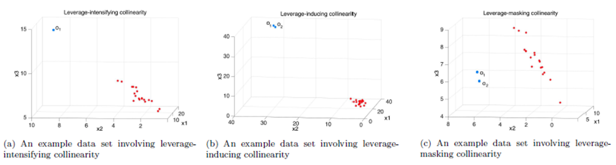 | Figure 1. Example data sets involving three types of collinearity-influential observations |
 | (3) |
 | (4) |
 | (5) |
 | (6) |
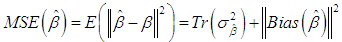
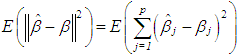
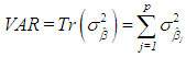
 is the estimate of
  and
and  is the variance of
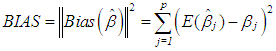
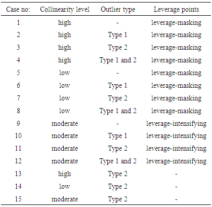
  is used. Tr is the trace operator and E is the expectation. Finding the most efficient estimator (by means of MSE, VAR and BIAS) for each case in Table 1 requires the knowledge of the following properties of the data: (1) ratio of outliers in data, (2) ratio of high-leverage points in data, (3) type of leverage points (masking, inducing or intensifying), (4) level of collinearity in data with and without the leverage points, (5) type of outlier(s) in data (Type 1, Type 2 or both). Thus, in Section 3.1, we will summarize our methodology by first describing the steps for generating synthetic data with known properties. Furthermore, the synthetic data will then be used to construct a lookup table that shows the estimator performance for each case in Table 1.
|
2. Estimators
- In this section we present the details of commonly used estimators compared in our simulation studies. First, we will describe the details of ridge estimators and summarize three of them using different ridge parameters. Second we will discuss five frequently used robust estimators - Least Median Square, Re-weighted Least Square, Least Trimmed Squares, M-estimator and S-estimator. Finally, we will present three ridge-type robust estimators.
2.1. Ridge Estimators
- The ridge regression estimator is introduced in [3] as,
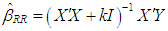 | (7) |
 | (8) |
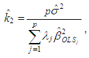 | (9) |
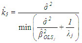 | (10) |
 is the jth eigenvalue of the matrix
  where
where  and
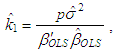
and  is given as follows
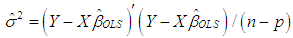 | (11) |
 in Equation (2). Henceforth,
  and
and  denote the ridge estimators computed by the ridge parameters
  and
and  respectively.
2.2. Robust Estimators
- In what follows, we describe frequently used robust estimators in literature to estimate parameter
 in Equation (1), [7,13,24].• Least median square (LMS)One of the most commonly used robust estimator is the LMS estimator, [13]. For our purposes, we summarize the steps of LMS algorithm as follows.Step 1: Generate all possible subsamples of observations with size p from n, and randomly select m subsamples out of all generated subsamples.Step 2: Perform regression analysis for m distinct subsamples (with size p).Step 3: For each regression compute the residual of ith observation where
  Step 4: Solve the objective function
 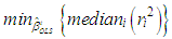 where
where  and
and  is the ordinary least square estimate
  for the tth subsample.Step 5: Finally,
  that minimizes the objective function is referred to as
  Furthermore, LMS estimate of the variance is calculated by
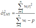 | (12) |
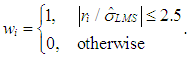 | (13) |
 ,
,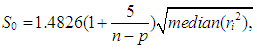 | (14) |
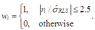
 in Equation (12).• Re-weighted least square (RLS)In order to compute RLS estimator [13], the goal becomes solving another objective function
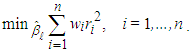 | (15) |
 is the well-known weighted least square estimator calculated from the
  iteration where and are the weight and residual for each observation, respectively. The
  that minimizes Equation (15) is defined as RLS estimator
  . The RLS estimator of variance is computed by
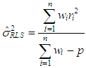 | (16) |
 | (17) |
 and associated residuals are used as initial conditions and
  is replaced by
  in Equation (17).• Least trimmed squares (LTS)For the LTS estimator, [13], we generate subsamples of data with size
 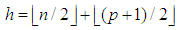 from n observations, where total number of subsamples is m and each subsample is enumerated as
  . For a subsample, we perform OLS regression analysis and compute residuals for n observations. Moreover, square of the residuals are ordered such that
 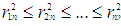 and
and  that minimizes
 | (18) |
 Note that when m is too large, a fixed number of randomly selected subsamples are used as an approximation to the optimal solution of
  for computational reasons. In [13], the details for finding the number of randomly selected subsamples are discussed for a desired probability of distance to the optimal value.• M-estimatorThis type of robust estimator is obtained from the solution of
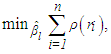 | (19) |
 computed at the
  iteration is defined as M-estimator,
  [24]. The details of the stopping rule that determines
  could be found in [24]. In the first iteration
  is used as the initial point and for the rest of the iterations weighted least squares is estimated by using
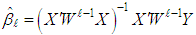 | (20) |
 is the current diagonal weight matrix with diagonal elements
  , [13]. In this study Tukey's bi-weight function
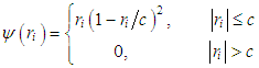 | (21) |
 and the weights
 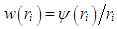 is used, [13]. Finally, in simulations the constant c is selected as 1.547 (the reason for this selection will be discussed in the following section)• S-estimatorS-estimator is proposed in [25] and it is computed by solving
 | (22) |
 is the estimate of the variance of the residuals. Here, in the iterative solution
  is also used as an initial point and
  obtained from the
  iteration is defined as S-estimator,
  To compute s, in each iteration, the equation
 | (23) |
 such that
  and
and 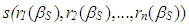 are asymptotically consistent estimates of
  and
and  for the Gaussian regression model and is usually taken as
  is the standard normal distribution. In this study, Tukey's biweight function (Equation (21)) is used with
  . This value is selected such that
  becomes 0:5 (breakdown point of S estimator), [24,25]. Same value of c is used in both S and M-estimator in order to be able to compare their performances.• Ridge-type robust estimatorsRidge-type robust estimator is proposed in [26] and it is computed by
 | (24) |
 is obtained by
 | (25) |
 and
and  can be selected as any type of robust estimator. In this study we use ridge-type RLS (RTRLS), ridge-type S (RTS), and ridge-type M (RTM) to compare their performances with the rest of the estimators presented above.
3. Simulations and an Example
- Here, we generate fifteen different synthetic data sets with varying levels of contamination. These data sets are then used to evaluate performances of twelve different estimators based on the Monte-Carlo estimates of total mean square, total variance and total bias. We show that these results can be used as lookup tables to select the best estimator for various cases of contamination. Moreover, we present an example to demonstrate an application of using these tables.
3.1. Simulations
- In this study, we generate contaminated normal distributed data with three explanatory variables
 that has the joint probability density function F for
  (in Equation (1)), where
  . Here,

 and
and  is the mixture parameter that satisfies
  , [24]. Here, the location parameters
  and
and  are used as design specifications. We parse them into elements such that
  and
and  where
where  and
and  , respectively.
  (or
(or  ) is the mean of
  for distribution
  (or
(or  ). Thus this parsing will allow us to use the set of design parameters
  to manipulate the level and the type of contamination corresponding to the cases presented in Table 1. In the simulations
  . To generate data with leverage-masking, leverage-inducing, and leverage-intensifying collinearity and are selected as•
 •
• 
 •
• 
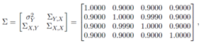
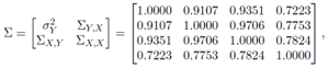 respectively. In order to generate data including leverage-masking collinearity, we use a covariance matrix with diagonal elements 1. Non-diagonal elements are close to 1 which guarantees strong collinearity between explanatory variables. Moreover, high-leverage observations drawn from the distribution
 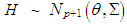 with
with  are added to data with ratio
  and
and  are estimates of
  computed from the observations generated from G and F, respectively. For instance, one may observe from Table 3 (Appendices) that even when
  is small
  is much smaller than
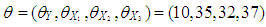
  Hence, a small number of high-leverage observations can mask the underlined strong collinearity associated with the majority of the data. In leverage inducing collinearity case, the covariance matrix has smaller non-diagonal elements and the corresponding
  (value computed from ) is smaller which implies no collinearity between explanatory variables. Similarly, high-leverage observations drawn from distribution H and with a different
  added to data with ratio
  In this case, we observe that
  value is much higher than
  computed without leverage points. This reveals that a small set of high-leverage observations can induce collinearity. A similar approach is taken for the third case of manipulation in which the high-leverage points intensify the strength of the collinearity.In what follows, we will describe the steps for generating data involving all combinations of contamination consisting of outliers and high-leverage points. Below, we list five manipulation methods used in our simulations.(1) The data (with size n) is generated by having only high-leverage points (masking, inducing or intensifying) with ratio
  . To achieve this, leverage points are drawn from the distribution
  and non-leverage points from
  . Then the observations of dependent variable for the leverage points are drawn from
  where
where  and
and  . Non-leverage points are also drawn from the same distribution
  by just replacing
  with
with  .(2) The data is generated by having only Type 1 outliers, which are also high-leverage points, with ratio
  . The observations of dependent variable associated with these leverage points are drawn from
  . Here,
  and
and  . Rest of the observations are drawn from
  where
where  and same variance
  .(3) The data is generated by having only Type 2 outliers with ratio
  that are drawn from
  where
where  and
and  . Rest of the observations are generated from
  where
where  and same variance
  (4) The data is generated by having both high-leverage points and Type 2 outliers with ratio
  . To achieve this, a combination of manipulations (1) for high-leverage points and (3) for Type 2 outliers is used. That is, leverage points are drawn from the distribution
  . Type 2 outliers with ratio
  are drawn from
  where
where 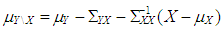 and
and  . Rest of the observations with ratio
  are generated from
  where
where  and same variance
  (5) The data is generated by having both Type 1 and Type 2 outliers each with ratio high-leverage points and Type 2 outliers with ratio
  . To achieve this a combination of manipulations (2) and (3) is used. For Type 1 outliers, we generate high-leverage points from
  with also ratio
  . The observations of dependent variable associated with these leverage points are drawn from
  . Here,
  and
and  . Moreover, Type 2 outliers are generated from
  with ratio
  where
where  and
and  . Rest of the observations with ratio
  are generated from
  where
where  and same variance
  Each manipulation is performed for leverage-masking, inducing and intensifying observations. Hence, in total there are 15 cases to be investigated as presented in Table 1 for which number of iterations is fixed to 10000 in order to compute the Monte-Carlo estimations of MSE, VAR, and BIAS given in Equation (4)-(6). Moreover, each case is investigated for various values of mixture parameter
  that contributes to the level of the manipulation. We present simulation results for the case when n = 50 and p = 3 since we observe that the results were similar for various
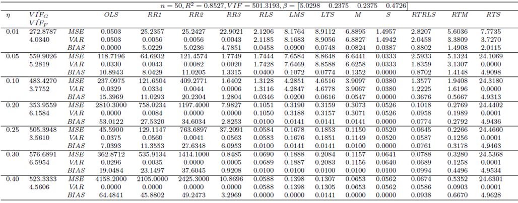
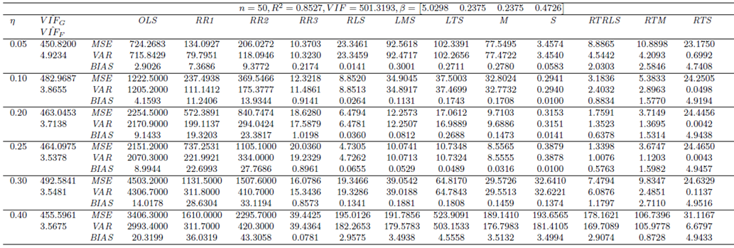
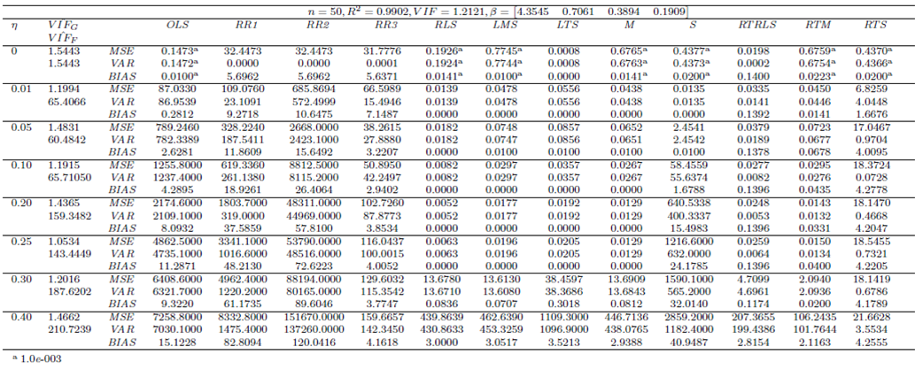
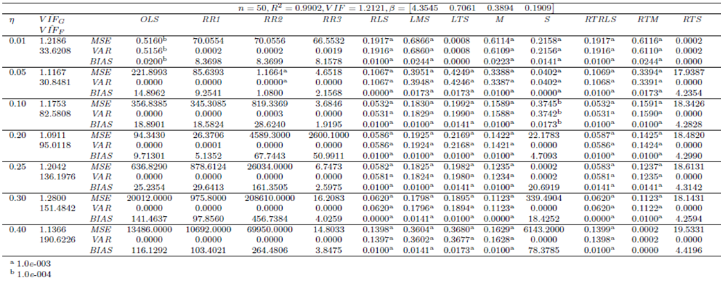
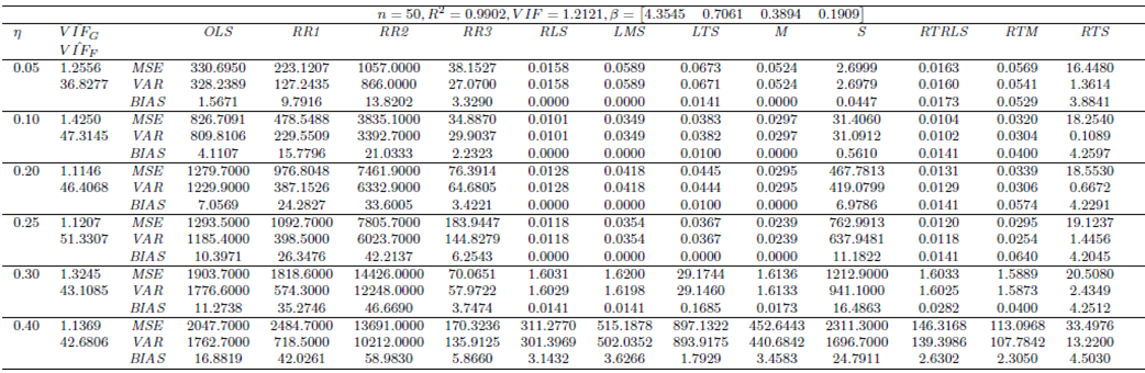
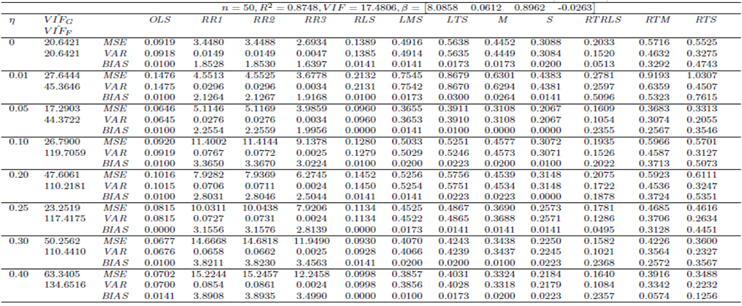
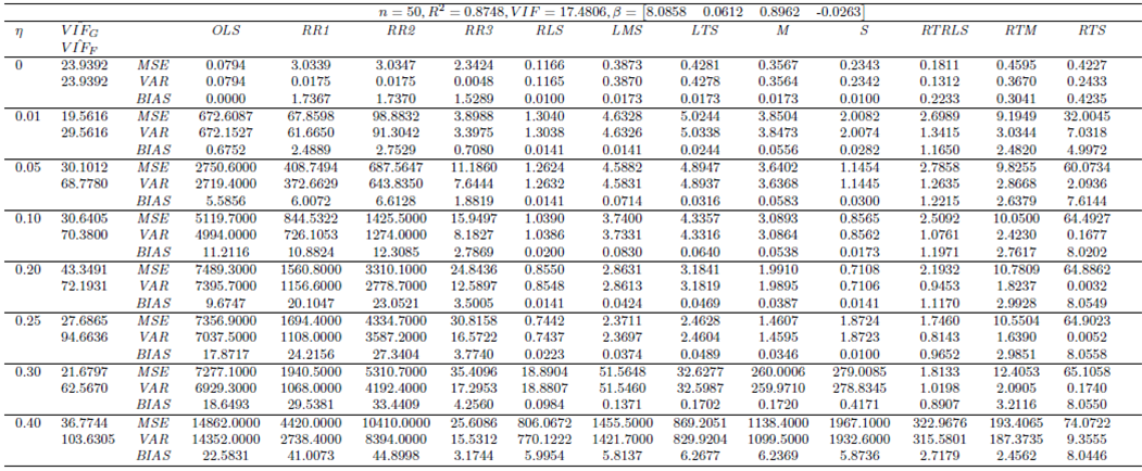
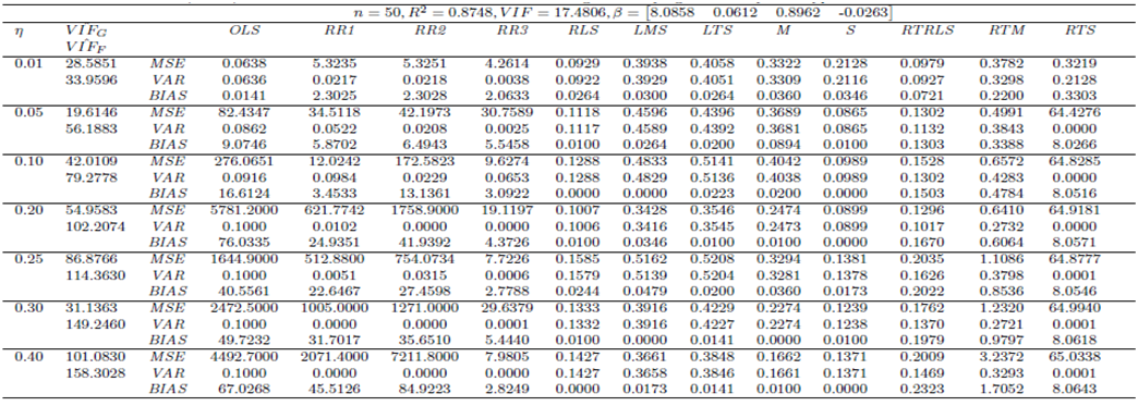
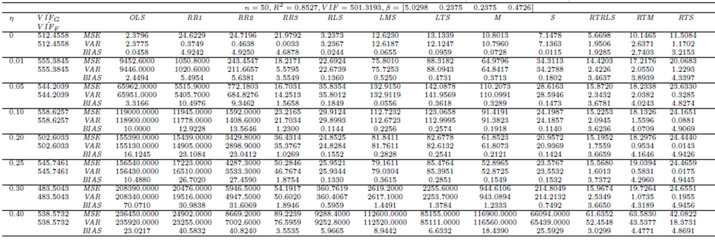
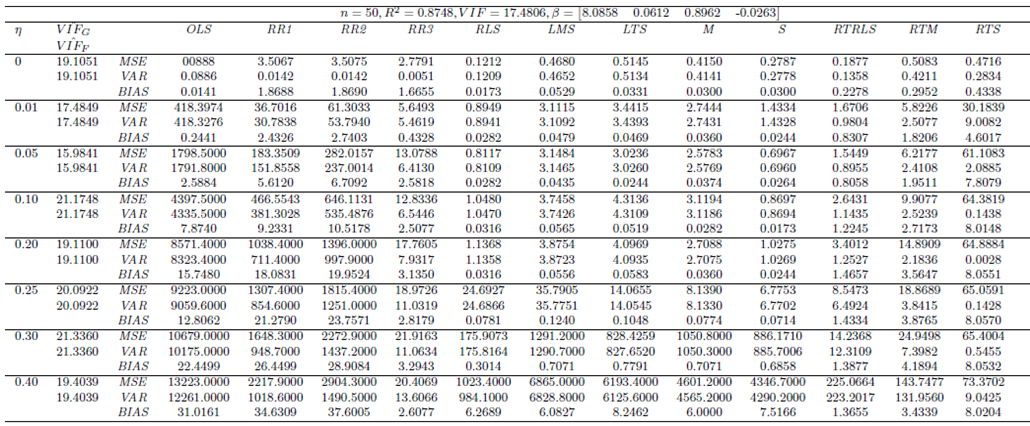
  combinations.Structurally, we first generate data with only leverage-masking collinearity associated with the cases 1 to 4 in Table 1 and present our results in Tables 3-6. (Appendices). Similarly, same steps are followed for leverage-inducing and leverage intensifying collinearity associated with the cases 5 to 8 and 9 to 12 in Table 1, and the results are shown in Tables 7-10 (Appendices) and 11-14 (Appendices), respectively. Finally, for the cases 13-15 in which estimator performances are compared when data has only Type 2 outliers with no leverage observations but relatively high, low and moderate level of collinearity the results are presented in Tables 15-17 (Appendices). In all of the Tables 2-17, OLS, RR1-RR2-RR3-RLS-LMS-LTS-M-S, and RTRLS-RTM-RTS denote the ordinary least squares, ridge, robust, and ridge-type robust estimators, respectively, presented in Section 2. Furthermore, in the top row of each table simulation parameters
  as well as the known
  value calculated from the covariance matrix are shown. In the second column of Tables 3-17,
  and
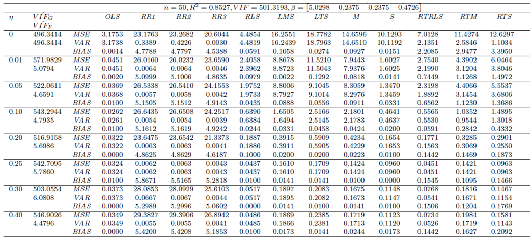
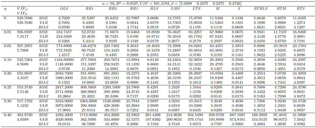
and  are computed from the first iteration of Monte-Carlo simulation in which the data is generated from G and F distributions, respectively. Each table presents the results based on MSE, VAR and BIAS computed by Equation (4)-(6).Let us first consider the cases when data only involves leverage observations. Figure 2a illustrates that the estimator RR3 (shown with red) performs the best based on variance. However, in a practical application, since
  value (computed from all of the observations, Table 3) is relatively small due the masking effect of leverage masking observations and there are no outliers, OLS (shown in blue) is expected to outperform the rest of the estimators, [6,8]. In contrast, in Figure 2c we observe that OLS performs the best even though ridge estimators (shown in red) are expected to perform the best for high
  value (Table 7) and no outliers [3]. Hence, we conclude that a small ratio of leverage-inducing observations in data causes a drastic increase in
  that is used to select estimators in practical applications. In Figure 2e there are only leverage-intensifying observations that strengthens an existing high level of collinearity (as one may observe from
  in Table 11) and we conclude that ridge estimator performs the best.If we observe Figure 2b and 2d a similar argument can be made for data that involves both high-leverage observations as well as outliers in X and Y directions. For instance, based on low
  value (Table 6) due to the masking effect of leverage masking collinearity, one may expect robust estimators to be the best performing estimator, [13]. However, Figure 2b illustrates that for varying range of mixture parameter ridge-type S estimator (RTS) outperforms the rest. Similarly, when the leverage observations induce collinearity (high
  value in Table 10), Figure 2d shows that robust estimator (RLS) performs better for
  This validates that observations classified as leverage-inducing collinearity are misleading since one expects ridge-type robust estimators to be more efficient for data sets with high collinearity and outliers [5,6].
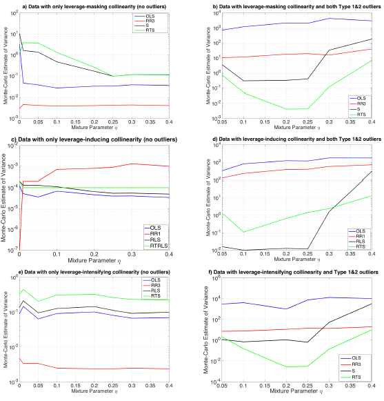 | Figure 2. 6 plots illustrating the logarithm of the Monte-Carlo estimates of variance as a function of mixture parameter η. Color coding in the figures is arranged such that OLS, ridge, robust, and ridge-type robust estimators are represented by blue, red, black, and green, respectively. The set of parameters used in each subplot (a)-(f) are presented in Tables 3, 6, 7, 10, 11, and 14, respectively |
 value should be computed by extracting the leverage points from the data for the best results. This suggests the use of robust
  calculations as we will discuss in Subsection 3.2. However, the precise contribution of robust
  computations to solve estimator selection problem is yet to be understood and this will be the subject of our future work. In Figure 3a-3c, we present results gathered from Tables 15-17, respectively. In Figure 3a, it is observed that ridge-type S estimator performs the best based on variance (RTS shown in green). Moreover, Figure 3b illustrates that for small values of
  robust estimators (RLS and S shown in black solid and dashed lines) but for higher values of
  ridge-type S estimator (RTS) has the lowest variance. Finally, Figure 3c, shows a similar trend around
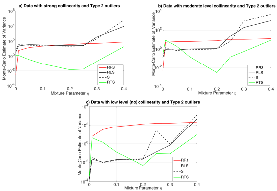 | Figure 3. 3 plots illustrating the logarithm of the Monte-Carlo estimates of variance as a function of mixture parameter η. Color coding in the figures is arranged such that ridge, robust, ridge-type robust estimators are represented by red, black and blue, green, respectively. The set of parameters used in each subplot (a), (b), (c) are presented in Tables 15, 17, 16, respectively |
3.2. Example
- In this section, we compare estimator performances (presented in Section 2) when they are applied to the data set introduced in [27]. This synthetic regression data is constructed such that there are three explanatory variables and in total
 observations that are enumerated from 1-75 such that the observations 1-10 are outliers in Type 1 direction
  Moreover, data is constructed such that the following 4 observations between 11 and 14 are leverage observations
  computed from 75 observations is 23.6842. This reveals that collinearity exists in data.
  obtained by excluding both outliers and leverage observations is found as 1.0163. Hence, we classify these (in total 15) observations as leverage-inducing collinearity. If we exclude only leverage observations and outliers,
  values are 34.1178 and 13.0166, respectively. These results indicate that Type 1 outliers induce collinearity more prominently than the leverage observations.Using this knowledge, one may use Table 8 (for data involving Type 1 outliers as well as leverage-inducing collinearity) which concludes that RLS estimator performs the best based on variance when mixture parameter is in the range
  . Moreover, for the same range of
  we observe from Table 8 that RLS and RTRLS have approximately the same value of VAR but RLS has lower BIAS and lower MSE values.In Table 2 (Appendices), we present results gathered from distinct methods to estimate the regression parameters for
 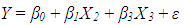 as well as
  values.
  is the estimate of
  . Moreover, it is computed by the set of observations used for calculating
  for each estimation method. In Table 2,
  value computed from RLS is equal to 13.0166. This is the same value computed by excluding only Type 1 outliers from data. Hence, this suggests that RLS estimator uses the subsample excluding all Type 1 observations which maximize its efficiency and this is in line with our results presented in Table 8.However, it is non-trivial to make the same conclusion for the rest of the robust estimators. Note that, since ridge estimators (RR1, RR2, RR3) use all the data their
  values (in Table 2) are found as 23.6842 which is estimated from the total data set with 75 observations. Ridge-type robust estimators RTRLS, RTM and RTS have the same
  values as RLS, M and S in that they use the same subsample.
4. Conclusions
- This study aims to construct a framework in order to compare estimator performances for various levels of contamination caused by collinearity, collinearity-influential observations and outliers in data. Furthermore, it targets to investigate the influence of their interactions by examining fifteen different data sets. These synthetically generated data sets involve distinct combinations of outliers classified as Type 1 or 2 based on their distance, and three distinct collinearity-influential observations, namely, leverage masking, leverage-inducing and leverage-intensifying collinearity. For the analysis, we use ridge, robust and ridge-type robust estimators from the literature and compute the Monte-Carlo estimates of total mean square, total variance and total bias for evaluating their estimation performances.We compare estimators based on variance and observe that when data involves high collinearity and only leverage-masking observations (no outliers), RR3 (ridge estimator) has the smallest variance. However, in a practical application due to the masking effect of the leverage observations,
 would be small and OLS estimator would be expected to perform the best for no collinearity and no outliers case, [6, 8]. Similar effects are observed when data involves leverage-inducing observations. Hence, we conclude that the interactions between collinearity and collinearity-influential observations can be misleading when selecting an estimator. These results reveal that
  , which is used for estimator selection, should be computed robustly by excluding the leverage points from the data set.We also observe that directionality in outliers and the strength of collinearity in data are also relevant for estimator selection. We show that the results presented in this study can be used as lookup tables to decide on the best estimator based on total variance, total mean square error and total bias values.
Appendices
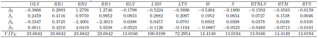 | Table 2. Parameter estimations and  values for the data values for the data |
 | Table 3. Case 1: MSE, VAR, BIAS and  values when data involves only leverage-masking collinearity (no outliers) values when data involves only leverage-masking collinearity (no outliers) |
 | Table 4. Case 2: MSE, VAR, BIAS and  values when data involves leverage-masking collinearity and Type 1 outliers values when data involves leverage-masking collinearity and Type 1 outliers |
 | Table 5. Case 3: MSE, VAR, BIAS and  values when data involves leverage-masking collinearity and Type 2 outliers values when data involves leverage-masking collinearity and Type 2 outliers |
 | Table 6. Case 4: MSE, VAR, BIAS and  values when data involves leverage-masking collinearity and Type 1 and 2 outliers values when data involves leverage-masking collinearity and Type 1 and 2 outliers |
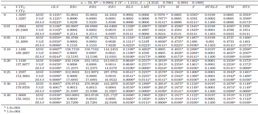 | Table 7. Case 5: MSE, VAR, BIAS and  values when data involves only leverage-inducing collinearity in data (no outliers) values when data involves only leverage-inducing collinearity in data (no outliers) |
 | Table 8. Case 6: MSE, VAR, BIAS and  values when data involves leverage-inducing collinearity and Type 1 outliers values when data involves leverage-inducing collinearity and Type 1 outliers |
 | Table 9. Case 7: MSE, VAR, BIAS and  values when data involves leverage-inducing collinearity and Type 2 outliers values when data involves leverage-inducing collinearity and Type 2 outliers |
 | Table 10. Case 8: MSE, VAR, BIAS and  values when data involves leverage-inducing collinearity and Type 1 and 2 outliers values when data involves leverage-inducing collinearity and Type 1 and 2 outliers |
 | Table 11. Case 9: MSE, VAR, BIAS and  values when data involves only leverage-intensifying collinearity (no outliers) values when data involves only leverage-intensifying collinearity (no outliers) |
 | Table 12. Case 10: MSE, VAR, BIAS and  values when data involves leverage-intensifying collinearity and Type 1 outliers values when data involves leverage-intensifying collinearity and Type 1 outliers |
 | Table 13. Case 11: MSE, VAR, BIAS and  values when data involves leverage-intensifying collinearity and Type 2 outliers values when data involves leverage-intensifying collinearity and Type 2 outliers |
 | Table 14. Case 12: MSE, VAR, BIAS and  values when data involves leverage-intensifying collinearity and Type 1 and 2 outliers values when data involves leverage-intensifying collinearity and Type 1 and 2 outliers |
 | Table 15. Case 13: MSE, VAR, BIAS and  values when data has high collinearity and Type 2 outliers (no leverage observations) values when data has high collinearity and Type 2 outliers (no leverage observations) |
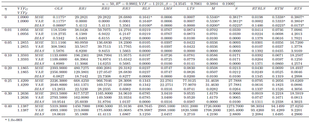 | Table 16. Case 14: MSE, VAR, BIAS and  values when data has low/no collinearity and Type 2 outliers (no leverage observations) values when data has low/no collinearity and Type 2 outliers (no leverage observations) |
 | Table 17. Case 15: MSE, VAR, BIAS and  values when data has moderate collinearity and Type 2 outliers (no leverage points) values when data has moderate collinearity and Type 2 outliers (no leverage points) |