1. Introduction

In many of the methods used for estimating the Factorial experiment models, such as classical Least Squares (LS), several assumptions are required such as normality, constant variances and independency. Those assumptions can be violated due to several causes, such as the presence of outliers observations, or non-normal data distribution. The last few decades there has been a growing interest in finding alternative ways to the classical methods, especially in applications that require asymmetric distributions (non-normal distributions). Also, many applications contain a large number of factors believed to be relevant in the study, but the actual effects of these factors are often few and unimportant. [1] discussed how to define extreme values in experimental design. It was known that the experiment outside the laboratory is an observation that with values that do not match the pattern of the values produced by the rest of the data. To address these problems, many researchers have proposed methods (or functions) used with LS, which are called "robust methods". Some of these methods are M-estimation, Huber function, [2], [3], etc. In [4] proposed the construction of a model using a B - technique and Box-Cox to data conversion or using General Linear Models (GLM) to eliminate the not normal data. The graphs were compared to the estimated responses through the length of the confidence interval for the mean responses in the design of industrial experiments. [5] introduced a new flexible regression model by considering an error term distributed according to the epsilon skew normal (ESN) distribution. In addition to the estimate of the classical parameters, the skewness parameter has been estimated.

In [6] the author introduced Robust Regression Shrinkage and consistent variable selection through the least absolute deviation (LAD)-Lasso, using the robust lasso with Huber loss function. The results of the study showed that the proposed method is resistant to outliers or heavy-tailed errors. In [7] proposed the modification of the 2ⁿ factorial experiments involving a Poisson response variable for comparison (Comparative Study of Analysis Factorial Experiments with a Poisson Distributed Response Variable, based on the criteria log-transformation (LOG), SQRT, ANOVA and GLM). The results of the study showed that the modified GLM approach exhibits the best performance with respect to all the three criteria in the entire parameter space and particularly so the expected response is likely to be very small. In [8] suggested using the general linear model (GLM) and log-transformation (LOG) for the purpose of experiments analysis. The response variable is non-normal distribution and the sample size is small. The work compared between the general linear model with log-transformation and ANOVA method on the basis of the results of the confidence limits and expected length confidence limits of E (LOCI) to the response variable which has an exponential distribution. [9] introduced the D-optimal design for when the error term in the simple linear regression follows the skew normal distribution. [10] utilized test Kraemer’s and Schaefer’s adaptive lasso on small samples and examined their effectiveness in designs with complex aliasing via simulations. In [11] introduced the case when the response variable follows the log-epsilon-skew-normal (LESN) distribution, which is an asymmetric probability distribution, and the parameters can be estimated using the maximum likelihood (MLE) method. The reliability for an experimental design that contains two factors with two levels, using simulation and real data are conducted to investigate the performance of the proposed method. The results show that the newly proposed method performs well.

In the present work we aim at combining the lasso variable selection and robust method (Huber loss function), for the analysis of the factorial experiment with two levels for each factor for the particular case when the response variable is distributed according to epsilon-skew-Laplace (ESL). Some concepts are explained in the relationship between factorial experiments and variables selection (factors). We also analyze two methods of variable selection – Lasso and adaptive Lasso. The simulation results indicated that this method gave acceptable results compared to Lasso and adaptive Lasso, depending on the criterion (MSE).

This paper is organized as follows. In Section 2 we present the fundamentals of the two level factorial experiments design and their advantages; in Section 3 we briefly introduce the concept of the epsilon-skew-Laplace distribution; in Section 4 we illustrate the variable selection and some methods (lasso, adaptive lasso) and the combination of the lasso variable selection with robust method (Huber function) for the analysis of factorial experiments when the response variable follows an ESL distribution. In Section 5 we summarize the results of a simulation study and present a data sample analysis. A brief conclusion is included in Section 6.

2. Two-level Factorial Experiment Design

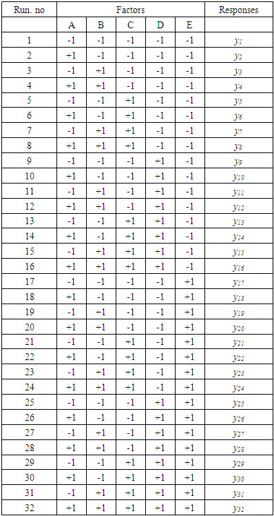
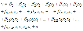
Factorial experimental designs are used for study the joint effect of a number of factors on a response variable at the same time. There are many cases of the factorial experiments design that are used in applied studies. One of these cases is when there are a number of factors (p) with two levels in experiment. A full factorial experiment of such a design requires 2×2…×2=2^p observations and is called a 2^p factorial experiment design [12]. The 2^p factorial experiment design is particularly useful in application fields such as medical, agricultural and industry, when there are many factors to be investigated. Therefore, these designs are used widely in these applications, because there are only two levels for each factor. In these designs we will refer to the levels as high and low, coded with +1 and -1, to denote the high and the low level of each factor. In most cases the levels are quantitative. Sometimes they are qualitative, such as gender, or two types of variety, brand, process or medical data.

This type of factorial experiment design has many methodological advantages:

It's orthogonal design that achieves the condition

X^TX=nl

where

X=(x_ij): design matrix and x_ij represents a factor j and level i.

I: identity matrix of the degree q×q

The estimates of parameter β_j (j=1, 2…, q) resulting from orthogonal designs are unbiased and have lower variances.

Finally, the orthogonal design matrix (X) achieves the possibility of measuring the main effects of the factors independently; the effects do not overlap with each other.

The possibility of estimating the interactions of the first order, the second, etc.

Results are appropriate for a large number of experimental conditions.

Our study will be limited to designs of type 2^p, which is one of the types of factorial designs in which p is chosen from the possible factors and then only two levels are assigned to each factor. The lower level is indicated by (-1) and the high level by (+1). The experiment model is implemented by representing 2^p of the factors, which allows us to estimate the main effects of factors X_j, (j = 1, 2, ..., p) as well as the possible interactions between the factors.

In this paper we use full factorial experiment consisting of five factors with two levels for each factor symbolized by 2⁵. The factors are expressed in capital letters A, B, C, D, and E. There are 2⁵=32 treatments or level combinations. Table 1. shows the full factorial design for five factors.

Table 1. The full factorial 25 design with two levels

The above table 1 shows the effect of the interaction indicating whether the influence of one factor depends on the levels of the other factors or not.

The analysis of experiments can be formulated in the form of the general linear regression [13]; [14]. A common regression model for studying the main effects and interactions is:

(1)

Here y is the response variable, the βs are unknown parameters, x₁, x₂, x₃, x₄, x₅ represent factors A, B, C, D and E, respectively, and ϵ is a random error term. The variables x₁, x₂, x₃, x₄, x₅, are coded as 1 and −1, for the high and low levels for their respective factors. The interaction between x₁ and x₂ is denoted as x₁x₂, and the other interaction effects are similarly defined. Often, when building a statistical model in the factorial experiments is desirable, the aim is to find a model to the estimated values for the response variable to be as close to the actual values as possible.

3. Epsilon Skew Laplace Distribution (ESL)

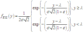
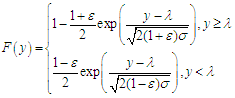
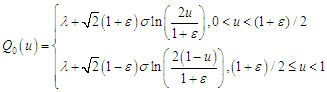
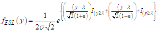
The random variable y has ESL distribution denoted by y~ ESL(λ,σ,ε), if there exist parameters λ ∈ R. σ>0, and -1<ε<1 such that the pdf of x is (Elsallouk, 2008) [21]:

(2)

where λ, σ and ε are location, scale, and skewness parameters, respectively.

The distribution function (cdf) of y is given by:

(3)

and the quintile distribution function of y is:

(4)

4. Variable Selection

4.1. Lasso Variable Selection Structure

The Lasso (Least Absolute Shrinkage and Selection Operator) is a linear model estimation method proposed by Tibshirani [16]. It refers to a group of methods that use an L₁ penalty to shrink parameter estimates and perform automatic variable selection. It is an L₁ penalised least squares regression. Like garrote, it shrinks some of the coefficients while setting the rest of them exactly to zero. Tibshirani considers the Lasso to be superior to ordinary least squares (OLS) regression for two reasons: Firstly, an over specified OLS model often has little bias but large variance, adversely affecting its prediction accuracy. This can be improved by shrinking or setting to zero some of the coefficients, trading some bias for a lower model variance. Secondly, OLS models may sometimes have a large number of small coefficients, adding little value to the model and complicating the interpretation of the effects.

The formally define the method for a linear regression model:

(5)

where Y=(Y₁, Y₂,…,Y_n )^r is the n dimensional vector of observed responses, X is the n × p. The design matrix, β=(β₁, β₂,…,β_p )^r is a p-dimensional vector of the unknown regression coefficients and ε=(ε₁, ε₂,…,ε_n)^r is the vector of random errors from a multivariate normal distribution N(0,σ²In). The columns of X are denoted as (X₁, X₂,…,X_P); these represent the p independent variables. The lasso estimate of β

(6)

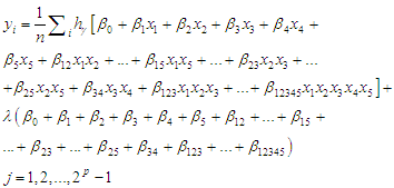
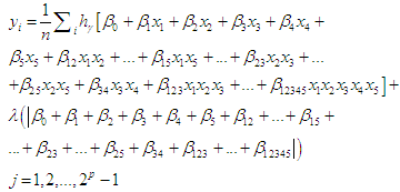
where is called lasso penalty.

In this work we can employ Lasso method in the equation (1) to factorial experiment model as follows:

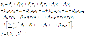(7)

For estimating the parameters in equation (7) we used the R program and the “Lasso2 package”, [15].

4.2. Adaptive Lasso Variable Selection

In [16] Zou introduced a new version of the Lasso method [16] based on the adaptive weights which in turn lead to different penalization and to different coefficients in the penalty. Adaptive Lasso, as a regularization method, avoids over fitting penalizing large coefficients. It has the same advantage as Lasso: it can shrink some of the coefficients to exactly zero. Zou [17] has given different weights to different coefficients. The adaptive lasso can be defined as:

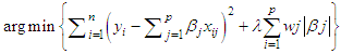(8)

where (w₁, w₂,…, w_p) are the adaptive weights. Zou [17] has shown that if the weights are efficiently chosen in a data-dependent way then the adaptive lasso can achieve the oracle properties. He suggested the use of estimated weights, , where β= {bj: j = 1, p} is a root-n-consistent estimator of β and γ > 0 is a user-chosen constant.

In this work we can employ adaptive Lasso method in the equation (1) to factorial experiment model as follows:

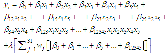(9)

For estimating the parameters in equation (9) we used the program R. “parcor” package, [18].

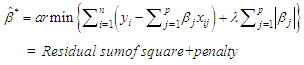
4.3. Robust Lasso Factorial Experiment When the Response Variable Follows the ESL Distribution

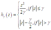
Many researchers developed methods of robust regression shrinkage with selection methods (like lasso). In [6] Wang introduced the robust regression shrinkage and consistent variable selection through the LAD-Lasso, using the robust lasso with Huber loss function. In this section, we attempt to develop an integrated methodology to combine the variable selection (Lasso) method and robust method (Huber loss function) for the analysis of factorial experiments with two levels for each factor when the response variables follow ESL distribution.

Suppose that the response variable, y, follows epsilon-skew-Laplace distribution. The probability density in equation (2) can be expressed as:

(10)

where λ represents the mean (location parameter) of the epsilon-skew Laplace, and ϵ

(11)

As we mentioned in the section (4.1), it can be solved by using the technique lasso for analysis factorial experiment of type 2⁵ design, as shown in equation (7).

Now, we will employ one of the robust methods (Huber loss function, 1973) also used by Yi and Huang, [19] in the regression models as follows:

(12)

where γ>0 is given constant. This function is quadratic for |z|≤γ and linear for |z|>γ.

As previously mentioned the Lasso formula used for factorial experiments analysis is given in the equation (7), and the Huber loss function of factorial experiment model is employed with Lasso variables selection. We can reach the following form:

(13)

where h_γ is the Huber loss function, and:

(14)

where 2^p-1=2⁵-1=31 which effects the factors. For estimating the parameters in equation (14) we used the program R and “hqreg” package [20].

5. Application

5.1. Simulation Study

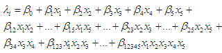
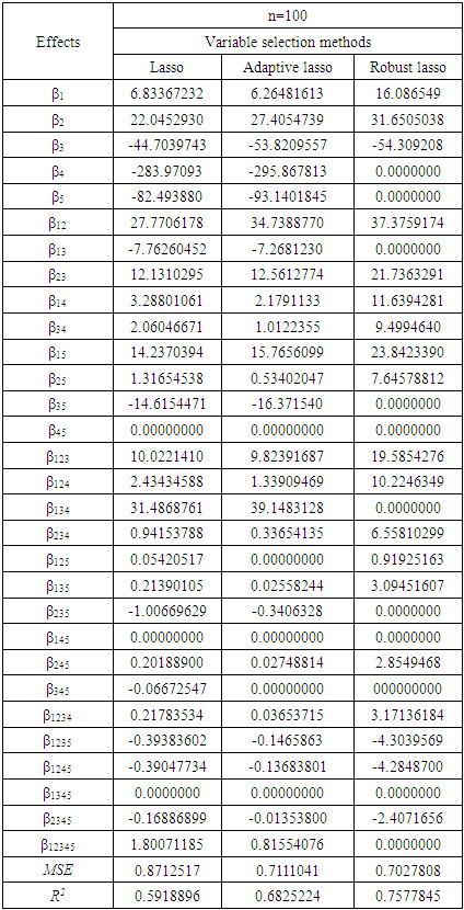
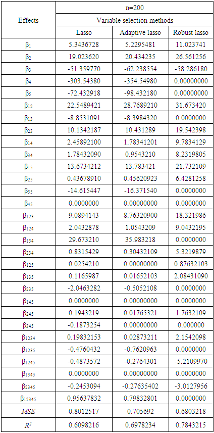
In this section, the simulation factorial experiments with non-normal responses which follow Epsilon-skew Laplace distributions are presented to illustrate the performance of the proposed approach. The simulation experiments are generated by the R program. The selected factorial experimental design is used to study five factors with two-level referred to as symbols A, B, C, D and E with interactions. For these factors, we represent the parameters (β₁, β₂,…β₁₂,…β₁₂₃₄₅). To compare the effectiveness of the robust lasso variable selection with lasso and adaptive lasso methods, we used the mean square error (MSE) to determine the most appropriate method for such data. For the model we used 1000 iterations generated for each combination of factors A, B, C, D, and E, represent by the parameters (β₁, β₂,…β₁₂,…β₁₂₃₄₅). Thee simulation of the program R is as follows:

Step 1: Generate the response data based on epsilon skew Laplace, using equation (4).

Step 2: For the lasso method, find the estimate parameter and selection variable (factors) using equation (7).

Step 3: For the adaptive lasso method, find the estimate parameter and selection variable (factors) using equation (9).

Step 4: For the robust lasso method, find the estimate parameter and selection variable (factors) using equation (14).

Step 5: Calculate the MSE and R Square (R²).

Table 2. and Table 3. summarize the results of the three methods (Lasso, adaptive lasso, robust lasso) for estimating and selecting factors to the factorial experiment model consisting of five factors with two levels for each factor. We can see that some parameters have zero for all three methods, but robust lasso method gave better results. This is evident through the mean square error simulation experiment, as the mean square error was less likely to compare with other methods. This indicates that the robust lasso method is more likely to be relevant in the explanation of the model and factors compared to the other methods mentioned earlier.

Table 2. Estimate and selection effects on simulation data for Factorial 25 analysis design (n=100)

Table 3. Estimate and selection effects on simulation data for Factorial 25 analysis design (n=200)

5.2. Method Illustration with Sample Data

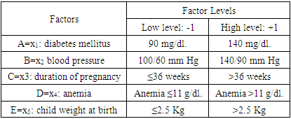
A sample data was collected from Women and Children Hospital in Diwaniyah in Iraq. The size of the sample included 64 cases of newborns of both sexes aged 1 to 10 days, all of these being children with early neonatal jaundice. The aim is to determine the most important factors leading to the disease of jaundice in newborns (Neonatal jaundice). The factorial experiments have been used to determine the most important factors affecting the percentage of jaundice in newborns, which represents the response variable (y) with the interactions of these factors at two levels for each factor: high level (+1) and low level (-1). There are 26 common factors are produced from the five main factors: diabetes mellitus of the mother, blood pressure, duration of pregnancy, mother anemia and child weight at birth. There are 10 two-factor interactions, 10 of the three-way interactions, 5 of the four-way interactions and one five-way interaction between the factors.

Table 4. Factors and levels for each factor

The main factors ant their interactions are detailed below:

a. Main Factors

A Diabetes mellitus – this factor has two levels: high level diabetes, the sugar level >140 mg/dl. And low level diabetes, the sugar level <90 mg/dl.

B Blood pressure - this factor his two levels: high level, the blood pressure level 140/90 mm Hg, and low level, the blood pressure level 100/60 mm Hg.

C Duration of pregnancy - this factor his two levels: high level, the duration of pregnancy >36 weeks, and low level, the duration of pregnancy ≤36 weeks.

D Anemia - this factor has two levels: high level, the anemia level >11 g/dl, and low level, the anemia level ≤11 g/dl.

E Child weight at birth - this factor his two levels: high level, child weight > 2.5 Kg, and low level, child weight≤2.5 Kg.

b. Two-factors interactions

ABTwo-factor interaction between diabetes mellitus and blood pressure.

ACTwo-factor interaction between diabetes mellitus and duration of pregnancy.

BCTwo-factor interactions between blood pressure and duration of pregnancy.

ADTwo-factor interaction between the diabetes mellitus and anemia.

BDTwo-factor interaction between blood pressure and anemia.

CDTwo-factor interaction between duration of pregnancy and anemia.

AETwo-factor interaction between the diabetes mellitus and child weight at birth.

BETwo-factor interaction between blood pressure and child weight at birth.

CETwo-factor interaction between duration of pregnancy and child weight at birth.

DETwo-factor interaction between anemia and child weight at birth.

c. Three-factors interactions

ABCThree-factor interaction between diabetes mellitus, blood pressure and duration of pregnancy.

ABDThree-factor interaction between diabetes mellitus, blood pressure and anemia.

ACDThree-factor interaction between diabetes mellitus, duration of pregnancy and the anemia.

BCDThree-factor interaction between blood pressure, duration of pregnancy and anemia.

ABEThree-factor interaction between diabetes mellitus, blood pressure and child weight at birth.

ACEThree-factor interaction between diabetes mellitus, duration of pregnancy and child weight at birth.

BCEThree-factor interaction between blood pressure, duration of pregnancy and child weight at birth.

ADEThree-factor interaction between diabetes mellitus, anemia and child weight at birth.

BDEThree-factor interaction between blood pressure, anemia and child weight at birth.

CDEThree-factor interaction between duration of pregnancy, anemia and child weight at birth.

d. Four-factors interactions

ABCDFour-factor interaction between diabetes mellitus, blood pressure, duration of pregnancy and anemia.

ABCEFour-factor interaction between diabetes mellitus, blood pressure, duration of pregnancy and child weight at birth.

ABDEFour-factor interaction between diabetes mellitus, blood pressure, anemia and child weight at birth.

ACDEFour-factor interaction between diabetes mellitus, duration of pregnancy, anemia and child weight at birth.

BCDEFour-factor interaction between blood pressure, duration of pregnancy, anemia and child weight at birth.

e. Five-factors interactions

ABCDEFive-factor interaction between diabetes mellitus, blood pressure, duration of pregnancy, anemia and child weight at birth.

y_i is the response variable, which represents the percentage of jaundice in newborns.

5.3. Data Analysis and Results

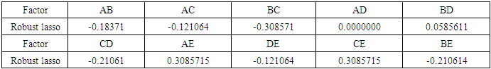
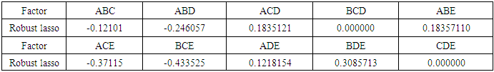
The data were analyzed using R program in order to determine the most important factors affecting the increase in the incidence of jaundice disease in newborns. We used the robust lasso variable selection method to determine the most important factors leading to the disease of jaundice in newborns. Data analysis results appear in a single table, but it has been divided into several tables for further clarification. Table 5., Table 6., Table 7., and Table 8. show the results obtained:

Table 5. Main effects (factors)

Table 6. Two-factor interaction

Table 7. Three-factor interactions

Table 8. Four and five-factor interactions

Main effects

The value for factor E (child weight at birth) are equal to zero, indicating that they are not significant and do not lead to the appearance of the disease of jaundice in newborns. We also note that A (diabetes mellitus), B (blood pressure), C (duration of pregnancy), and D (anemia) represent the main factors having major effects and leading to the appearance of the disease of jaundice in newborns.

Two-factor interactions

Through the results of Table 6 we note the interactions AD (diabetes mellitus and anemia) we observe that their value are equal to zero. This indicates that they are not significant and do not lead to the appearance of the disease of jaundice in newborns. We also note that factor interactions AB (diabetes mellitus and blood pressure), AC (diabetes mellitus and duration of pregnancy), BC (blood pressure and duration of pregnancy), BD (blood pressure and anemia), CD (duration of pregnancy and anemia), AE (diabetes mellitus and child weight at birth), DE (anemia and child weight at birth), CE (duration of pregnancy and child weight at birth) and BE (blood pressure and child weight at birth) have significant effect and lead to the appearance of the disease of jaundice in newborns.

Three-factor interactions

From the Table 7, we find that the values of interactions BCD (blood pressure, duration of pregnancy and anemia) and CDE (duration of pregnancy, anemia and child weight at birth) have values equal to zero. This indicates that they are not significant and do not lead to the appearance of the disease of jaundice in newborns. We also note that factor interactions ABC (Diabetes mellitus, blood pressure and duration of pregnancy), ABD (diabetes mellitus, blood pressure and anemia), ACD (diabetes mellitus, duration of pregnancy and anemia), ABE (diabetes mellitus, blood pressure and child weight at birth), ACE (diabetes mellitus, duration of pregnancy and child weight at birth), BCE blood pressure, duration of pregnancy and child weight at birth), ADE (diabetes mellitus, anemia and child weight at birth) and BDE (blood pressure, anemia and child weight at birth), have significant effect and lead to the appearance of the disease of jaundice in newborns.

Four and five -factor interactions

Table 8. presents the results of four-factor interactions, from the results we can see that the ABCE (Diabetes mellitus, blood pressure, duration of pregnancy and child weight at birth) and ABDE (diabetes mellitus, blood pressure, anemia and child weight at birth) has the value equal to zero, indicating that it is not significant and does not lead to the disease of jaundice in newborns. We also note that the factor interactions ABCD (diabetes mellitus, blood pressure, duration of pregnancy and anemia), ACDE (diabetes mellitus, duration of pregnancy, anemia and child weight at birth), and BCDE (blood pressure, duration of pregnancy, anemia and child weight at birth) have significant effect and lead to the disease of jaundice in newborns. And also we can note that the value of five-factors interactions (ABCDE) (diabetes mellitus, blood pressure, duration of pregnancy, anemia and child weight at birth) has the value different than zero. This means that it is significant and leads to appearance of the disease of jaundice in newborns.

6. Conclusions

In this paper we have presented a new methodology to analyze factorial experiments when the response variable follows epsilon skew Laplace distribution. We employed a Huber function with lasso variable selection (robust lasso), through the results simulation and real data. We observed that the proposed method (robust lasso) gave better results than lasso and adaptive lasso methods. This inference is clear from the results of the MSE and R squared in the simulation experiments as well as in the results of the application of real data, we observed that the robust lasso method can be used to estimate and select all five main effects, all 10 two-factor interactions, 10 three-factor interactions, 5 four-factor interactions and one five-factor interaction. Through the obtained results, we have reached a set of results pertaining to the study of the influence of the main factors and interactions that lead to the disease of jaundice in newborns and the significant factors with interactions are:

a. Main effects for factors

A (diabetes mellitus), B (blood pressure), C (duration of pregnancy) and D (anemia).

b. Two-factor interactions

Interactions factors AB (diabetes mellitus and blood pressure), AC (diabetes mellitus and duration of pregnancy), BC (blood pressure and duration of pregnancy), BD (blood pressure and anemia), CD (duration of pregnancy and anemia), BE (blood pressure and child weight at birth), AE (diabetes mellitus and child weight at birth), CE (duration of pregnancy and child weight at birth) and DE (anemia and child weight at birth).

c. Three-factor interactions

Interactions factors ABD (diabetes mellitus, blood pressure and anemia), ABE (diabetes mellitus, blood pressure and child weight at birth), ACD (diabetes mellitus, duration of pregnancy and anemia), ABE (diabetes mellitus, blood pressure and child weight at birth), ACE (diabetes mellitus, duration of pregnancy and child weight at birth), BCE blood pressure, duration of pregnancy and child weight at birth), ADE (diabetes mellitus, anemia and child weight at birth) and BDE (blood pressure, anemia and child weight at birth).

d. Four and five-factor interactions

Interactions factors ABCD (diabetes mellitus, blood pressure, duration of pregnancy and anemia), ACDE (diabetes mellitus, duration of pregnancy, anemia and child weight at birth) and BCDE (blood pressure, duration of pregnancy, anemia and child weight at birth) have significant effect and lead to the disease of jaundice in newborns. And also we can note that the value of five-factors interactions (ABCDE) (diabetes mellitus, blood pressure, duration of pregnancy, anemia and child weight at birth).