1. Introduction

Thalassemia is an inherited disease that is transmitted from parents to children across genes and affects the ability to produce hemoglobin in the human body, leading to severe anemia. The most common type is found among children with anemia in all parts of world. This disease is caused by genetic acquired factors. Iron deficiency anemia affects a large number of children, and significantly more than other types of anemia in poor and developing countries, where there is an increased incidence of some infections [1]. The World Health Organization has calculated that about 7% of the world’s population carry a hemoglobinopathy gene [2]. In the Mediterranean area, there are 15 to 25 million of healthy carriers [3]. Iraq is one of the countries with health, environmental and economic difficulties [4]. The statistics announced by government agencies on blood diseases confirmed high rates of patients with Thalassemia in the last few years, especially among children. The increase in the incidence of infection is due to several reasons, including the remnants of war and its impact on generations as well as the genetic factor and lack of health awareness among people.

Statistics show that the of Thalassemia patients has increased significantly in recent years. After the 2003 war that the rates of this genetic blood diseases in children in Iraq has risen to 22 cases per 100 thousands children compared with 2002, when it only appeared in 4 children out of 100,000 children. This number is much higher compared to neighboring countries. Children with Thalassemia need a life-long treatment of regular blood transfusion and iron chelation. Thalassemia has negative impact on many aspects of the life for children.

Thus, it is necessary to acknowledge the causes of the disease and the variables that cause infection with the disease. In this case, the Quantile regression models help define the relationship between a set of proposed predictor variables and the specific quantiles of the response variables analogous to a linear regression, which investigate the mean value of the response variables for a given set of predictor variables [5]. Quantile regression leads to a more comprehensive analysis by estimating the changes in specific quantiles of the response variables with respect to predictor variables, providing relationship at different points in the conditional distribution of the response variable. Since the pioneering research of Koenker and Bassett [6], quantile regression models have been the topic of major theoretical interest as well as many practical applications in many different areas such as: economics, survival analysis, microarray study, growth chart, finance, biomedical studies. A comprehensive account of these recent applications can be found in Koenker [7], and Cade and Barry [8]. The ridge parameter in quantile regression is employed to address the most important challenges that may arise with medical data, such as multicollinearity [9]. This problem arises because of the high correlation between the independent variables that lead to weak estimates. It is important to note the fact that in analysis of factors affecting the incidence of Thalassemia, the variables in the phenomenon under study are linked to each other in one way or another, either directly or indirectly. The existence of these relationships have several effects on the results of the analysis obtained. Nevertheless, existing literature shows that this issue is not adequately addressed.

Many researchers have pursued different aspects and ways of solving multicollinearity. In 1975, Hoerl and Kennard developed a new method by adding a positive value (k) to the elements of the information matrix, the so called ridge parameter [10].

The ridge estimator is used to solve the identification problem that can be viewed from a Bayesian perspective (Congdon, [11]). In this paper we will use Bayesian methods to choose the ridge parameter.

In 2013, Cule, E. and De Iorio, M. identified numerous genetic associated with diverse phenotypic traits. However, the identified associations generally explain only a small proportion of trait heritability and the predictive power of models incorporating only known-associated variants has been small, considering the joint effect of many genetic variants simultaneously. The study found ridge regression, a penalized regression approach that has been shown to offer good performance in multivariate prediction problems [12].

The variance is higher in the OLS method if in the multiple regression model, the linear correlation between explanatory variables is high [13]. The results of this study were obtained by using ridge regression study. Also, the authors showed that the best results are achieved with the ridge regression method of Hoerl and Kennard’s. Bager et al. (2017) aimed to determine the most important macroeconomic factors which affect the unemployment rate in Iraq by using a ridge regression method, one of the most widely used methods for solving the multicollinearity problem [14].

This paper aims to use the ridge parameter in the quantile regression to address important challenges, such as the multicollinearity problem. A Bayesian method is used for estimation of the ridge parameter in quantile regression. Because this technique could provide an important research tool, it may help to find the most appropriate value for the parameter. The paper would also contribute to develop a robust statistical model to identify the most important factors affecting patients with thalassemia across various quantile ratios. The model helps rank the relevant factors affecting patients. The findings of the study can be potentially useful for the identification of the causes of the disease in order to reduce its incidence.

The paper structure is the following: section two provides ridge regression method, section three includes the ridge and quantile regression models, section four covers the test of the multicollinearity problems, section five is the application to the case study and section six includes the conclusions.

2. Ridge Regression Method

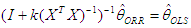
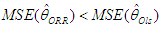
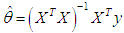
The history of multicollinearity dates back at least to the paper of Frisch (1934) who introduced the concept in order to describe a situation where the variables dealt with are subject to two or more relations. One way to approach this problem is called the ridge regression, first introduced by Horel and Kennard [15] who suggested an alternative method to the standard method of ordinary least squares (OLS). The ordinary ridge regression method (ORR) has become one of the most applied solutions for addressing the problem of semi-multicollinearity.

The method implies adding a small positive constant (K) to the main diagonal elements of the information matrix (X^TX). This positive value, known as the ridge parameter, decodes the links between the explanatory variables. The ORR method can be written as follows:

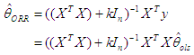(1)

k>0: ridge parameter in identity matrix

When 𝑘=0, the ordinary ridge regression method converts to the ordinary least square method.

(2)

When introducing the ridge parameter k, the variation of estimated parameters is reduced. Although the ordinary ridge regression method is biased, it produces a mean square error (MSE) lower than the mean square error obtained with OLS method.

(3)

The ridge estimator is regarded as the minimize of the residual sum square as the following formal (Tibshirani, [16]):

(4)

3. Ridge and Quantile Regression Models

In quantile regression there should be no multicollinearity in predictor variables. We will address this problem by using the ridge regression which can overcome the multicollinearity problem. An optimum ridge coefficient can be estimated through many methods. The quantile regression model has the following form [7]:

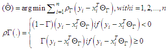(5)

The quantile regression with ridge regression use the ridge coefficients to build the quantile regression model. The solution of the ridge coefficient can be written as the following equation [17]:

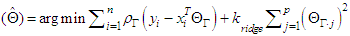(6)

where (k) ridge parameter.

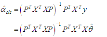
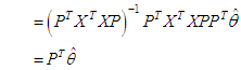
3.1. Estimator Parameter (k)

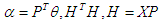
The multiple linear regression model can be expressed as:

(7)

where:

Y: Represents the vector of the dependent variable with dimension (n × 1)

x: Represents the vector of the independent variable with dimension (n × p)

θ: Represents the vector of parameter regression with dimension (P × 1)

ε: Represents the vector of random error with dimension (n × 1).

The ordinary least square estimator (OLS) of the regression coefficients θ is defined as [18]:

(8)

Suppose the diagonal matrix has the orthogonal conversion p; it results that and the matrices p and Λ are matrices eigenvalue and eigenvector for matrix . 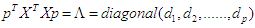where d_i is the eigenvalue of number j of the matrix and 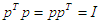. The orthogonal (canonical form) version of the multiple regression model (7) is [19] [20]:

(9)

Where:

(10)

(11)

(12)

Then the estimator .

From equation (8) we can write:

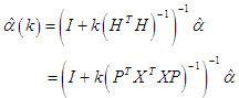where: .

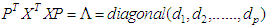The equation above simplified:

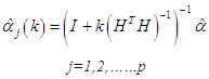(13)

From the above equation the value (k) can be chosen [21].

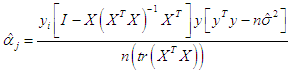
3.2. Bayesian Approach to Estimator Parameter (k)

Ridge regression has a close connection to Bayesian linear regression. The first review of the Bayesian derivation and interpretation of the ridge estimator along the line was provided by Loesgen [22]. The ridge estimator proposed to solve the identification problem can be viewed from a Bayesian perspective [8]. To the estimate ridge parameter, we depend on the result. Lindely and Smith [19] express the formula into Bayesian for estimating the linear regression model through an appreciation multi stages and use multivariate normal prior distribution when the parameter is unknown at every stage of the analysis. In this case, the prior is considered to be marginal distribution: .

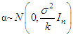The posterior distribution can be rewritten to depend on Bayesian estimator k as follows [1], [23]:

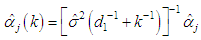(14)

where

(15)

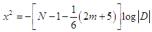
4. Test Multicollinearity Problems (Farrar & Glauber Test)

This test is based on a Chi square test (x²) to determine whether or not there is a multicollinearity problem in the estimated model.

The test formula is:

(16)

where:

N: represents the sample size.

m: represents the number of explanatory variables.

log|D|: represents the normal logarithm to determinant the correlation matrix.

Then we compared between the table values in a degree of freedom ((m(m-1)) ⁄ 2) and specific significance level. The null hypothesis is rejected if the calculated value is greater than the tabular value. It isn't rejected if the calculated value is smaller than the tabular value [24].

5. The Sample and Data Analysis

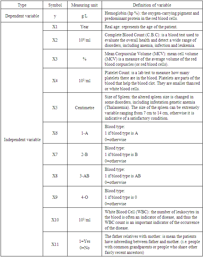
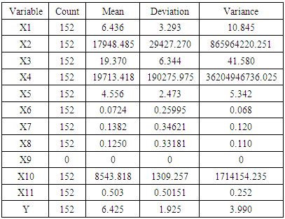
The inasmuch prevalence of genetic blood diseases (Thalassemia) varies among areas of Iraq with the highest incidence of infections in the middle Al-Forat region and southern Iraq, according to the Iraqi Ministry of Health (National Cancer Council). This study was conducted to determine the factors affecting the children infected with some genetic anemia (Thalassemia). The sample was taken for 152 patients from centers for the treatment of blood diseases in that areas during 2016. This paper used the quantile regression model at four quantile levels (0.25, 0.50, 0.75, 0.95) respectively, because quantile regression has attractive properties. The variables that are thought to affect the disease were selected after the consultation of doctors specialists and practitioners in genetic anemia (Thalassemia). The following table (Table 1) describes the variables:

Table 1. Descriptive variables

Table 2. Descriptive statistics

The Table 2. above shows the descriptive statistics of the variables of the model, in order to describe the nature of the variables under study. The following is an analytical presentation of these measures for each variable of the model. Show that the mean age patients in the sample was 6.43 years with the standard deviation 3.293 years, while the variance is 10.845 years. The results also show that the mean value for the complete blood count (C.B.C) was 17984.485(10⁶/ml) and a deviation 29427.270(10⁶/ml), while the variance 865964220.251(10⁶/ml).

The mean corpuscular volume (M.C.V) is 19.370%, while the deviation was 6.344% and the variance 41.580%. The results also show that the mean value for the mean corpuscular volume (M.C.V) was 19713.418(10³/ml) and a deviation 190275.975(10³/ml). Mean size of spleen in the sample was 4.556c.m, with the deviation 2.473c.m, while the variance 5.342c.m. The results of the descriptive statistics show that the mean of the white blood cell (W.B.C) was 8543.818(10³/ml) and a deviation was 1309.257(10³/ml).

Finally, the mean the fathers’ relatives with mothers was 0.503 that is mean about half of the patients have inbreeding between father and mother.

5.1. Testing the Multicollinearity Problems

We calculated the Chi square test (x²). To apply this test, these steps were followed:

a. test hypothesis:

H₀=X_J nonexistence multicollinearity problem

H₁=X_J existence multicollinearity problem

b. calculate the Chi- square test (x²):

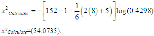(17)

By comparing the calculated value to the tabular value, it is evident that it is greater, leading to rejection of null hypothesis and acceptance of alternative hypothesis, thus, proving that the model suffers from multicollinearity problem. Therefore, the parameters of the quantile regression model cannot be estimated directly, because the estimation will be inaccurate. First, the issue must be treated by using the ridge regression method.

5.2. Determine the Causative Variables of the Multicollinearity Problems

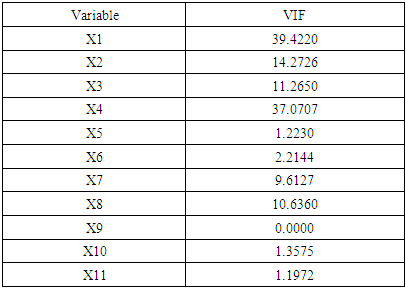
In order to determine the variables causing the problem of linear multiplicity the Variance Inflation Factor (VIF) will be used, which measures the inflation of the parameter estimates for all explanatory variables in the model. These indicators were computed for the regression parameters of all the explanatory variables of the model. The multicollinearity between the explanatory variables was determined with the following results:

Table 3. Variance Inflation Factors (VIF)

We notice from Table 3 that the values of the VIF for some of the explanatory variables (X1, X2, X3, X4, X8) are greater than 10, this means on the presence of the multicollinearity problem between explanatory variables.

5.3. Ridge Quantile Regression Analysis

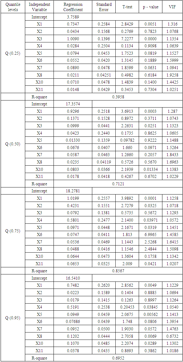
This method allows the estimation of the quantile regression models established by ridge coefficients. These coefficients are selected based on the Bayesian method for parameter (k) estimation. This method was used to find the best value of the ridge parameter in accordance with formula (15). Using R package the following result was reached: 𝑘 = 0.02578. Table 4 shows the results for each quantile coefficients.

The results presented in Table 4. for the coefficient estimation at the quantile levels 0.25, 0.50, 0.75 and 0.95 show the following:

a. At the quantile level (0.25): the variables X1 and X3 have a significant effect on the dependent variable according to p-value and R-square (0.3958); this means the independent variables can explain 39.5% of the variation in the dependent variable. This quantile level is weak in interpreting the data of the phenomenon under study. The VIF values for X1 and X3 are 1.1316 and 1.1354, respectively. That is an indicator that the multicollinearity problem is solved.

b. The results were quantile level 0.50 showed that the variables X1, X3, X10 have a significant effect on the dependent variable. The R-square value (0.7121) indicates that the independent variables can explain 71.2% of the variation in the dependent variable. This level is also weak in interpreting the data of the phenomenon under study. The VIF values for X1, X3, X10 are 1.2870, 1.1323 and 1.1383, respectively. This is an indicator that the multicollinearity problem is solved.

c. The results at the quantile level 0.75, indicate that the variables X1, X2, X4, X5 and X11 have a significant effect on the dependent variable (Incidence of anemia in children, Thalassemia). The R-square (0.8567) shows that the independent variables, can explain 85.6% of the variation in the dependent variable. This quantile level is strong and the variables have a direct correlation with the response variable except three variables (X3, X6, X7, X8 and X10). These variables have weak effect according to this measure, all the results are logical by the medical side. The VIF values for X1, X2, X4, X5 and X8 are 1.1258, 1.0718, 1.057, 1.1451, and 1.0207. This indicates that the multicollinearity problem is solved.

d. At quantile level 0.95, the variables X1, X5, X8 and X10 have a significant effect on the adopted variable. The value of R-square (0.6952) shows that the independent variables can explain 69.5% of the variation in the independent variable. This ratio is small and can't be used to interpret the results.

Finally, the last step of our analysis is to compare the performance of the quantile levels in ridge quantile regression. This comparison would help to better select the best quantile level. Through comparison we found that the quantile level at 0.75 is the best as it has a high R-square (0.8567) according to the interpretation of the data regarding the phenomenon under study.

Table 4. Ridge quantile regression analysis

6. Conclusions

In this paper, the multicollinearity issues in quantile regression models were the subject under research, in an attempt to find practical solutions to deal with the violation issue of a regression model assumption. The solution adopted in our research is the ridge regression and for estimating the parameter of the ridge we use the Bayesian approach. We tested this approach for identifying the factors affecting anemia in children (Thalassemia) across various quantile ratios.

The study showed that the use of the ridge quantile regression method in the cases when the independent variables are affected by multicollinearity is one of the successful ways to solve this issue. Therefore, applying the ridge quantile regression method in other studies is recommended, since it provides better estimators than the ordinary regression methods when the independent variables are related, without omitting any of the independent variables.

By applying the ridge regression method at quantile level 0.75, we found that there were five variables with a significant impact on the anemia in children (Thalassemia) in Iraq at the statistically significant level less for 0.05%: real age, complete blood count, platelet count, size of spleen, the relatives between father and mother, where was the p-value as (0.0001, 0.0325, 0.03971, 0.0319, 0.0421) respectively. As for the rest of the variables (mean corpuscular volume, Blood type, white blood cell) the study shows that they are weak and have no significant statistical effect.

The results are explained by the fact that Iraq is one of developing countries still facing health, environmental and economic difficulties.

ACKNOWLEDGEMENTS

The author wishes to acknowledge the contribution of all the physicians that helped collecting and analysing the data for this study.