-
Paper Information
- Next Paper
- Previous Paper
- Paper Submission
-
Journal Information
- About This Journal
- Editorial Board
- Current Issue
- Archive
- Author Guidelines
- Contact Us
International Journal of Statistics and Applications
p-ISSN: 2168-5193 e-ISSN: 2168-5215
2018; 8(2): 53-58
doi:10.5923/j.statistics.20180802.03

Analysis of Nigeria Stock Market Using Bayesian Approach in Stochastic Volatility Model (2012 – 2016)
 Abstract
 Reference
 Full-Text PDF
 Full-text HTML
Yakubu Anjikwi 1, Jibasen Danjuma 2
1Department of Agricultural Economics, University of Maiduguri, Maiduguri, Nigeria
2Department of Statistics and Operations Research, School of Physical Science, Modibbo Adama University of Technology Yola, Yola, Nigeria
Correspondence to: Yakubu Anjikwi , Department of Agricultural Economics, University of Maiduguri, Maiduguri, Nigeria.
| Email: |  |
This work is licensed under the Creative Commons Attribution International License (CC BY).
http://creativecommons.org/licenses/by/4.0/

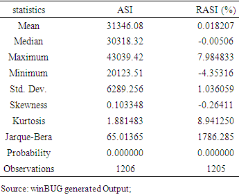
This research was conducted to analyzed volatility in Nigeria stock market using Bayesian approach in stochastic volatility model. The sample data used for this study were daily and weekly closing prices of All Share Index over the period of January 30th, 2012 to December 8th, 2016. The analysis was carried out based on posterior credible interval estimates produced by running MCMC algorithm for 10,000 iterations, with a burn-in of 1000000 and the first 1000 iterations discarded. The result of the study revealed evidence of significant variation in the price movement, as shown by the large differences between minimum (-4.35316) and maximum (7.984833) with mean estimate (0.018). The result for unit root test based on Posterior means and 95% posterior intervals for  and
and  shows that there is a significant evidence for unit-root in log- volatility model for All share index (the corresponding 95% posterior intervals include the point 1) i.e [0.9995,1.0]. The inter-correlation among the Posterior parameters revealed that there is a less or no collinearity between the parameters of estimate. Mean estimate for
  were found to be 0.7504 and 2.286 respectively for daily and weekly share price, indicating volatility clustering in the series. The study that revealed volatility persistence were significantly high with mean estimated close to unity for daily and weekly series respectively. The estimate for leverage parameter showed -0.566 and -0.561 for daily and weekly respectively. Arising from this study, stochastic volatility model could be used to test price movement in Nigerian stock market to make it better utilized by financial experts, econometrician and researcher.
Keywords: Nigerian Stock Market, Volatility Clustering, Stochastic Volatility Model, Unit Root, Prior Distribution
Cite this paper: Yakubu Anjikwi , Jibasen Danjuma , Analysis of Nigeria Stock Market Using Bayesian Approach in Stochastic Volatility Model (2012 – 2016), International Journal of Statistics and Applications, Vol. 8 No. 2, 2018, pp. 53-58. doi: 10.5923/j.statistics.20180802.03.
1. Introduction
- All over the world, capital market segment of the financial market plays a vital role in the process of economic growth, through the mobilization of long term funds for future investment. A well-functioning stock market fosters growth and profit incentives and helps in risk management more efficiently than the bank-based system does [34] and [29]. [30] expounds theoretically that a more developed stock market may provide liquidity that lowers the cost of the foreign capital essential for development, especially in low-income countries that cannot generate sufficient domestic savings. [35], [33] and [28] envisaged that stock market development is vital for economic growth. The fluctuation of general stock market index expresses the level of economic growth, the degree of trade openness and the financial depth in a developing or developed country. In Nigeria, for instance, the stock market helps in long term financing of government development projects, serves as a source of fund for private sector long term investment and served as a catalyst during the 2004/2005 banking system consolidation. Market capitalization as a percentage of nominal Gross Domestic Product (Nominal GDP) stood above 100% from 2007 to 2008, reflecting high market valuation and activities. However, according to [31] statistical Bulletin, the All Share Index (ASI), which shows the price movement of quoted stocks moved from 61,833.56 index points in the first quarter of 2008 to 20,244.73 index points in fourth quarter of 2011, suggesting some level of fluctuations in the stock market, especially since the occurrence of the 2008/2009 financial crisis.An increase or decrease in the value of stock tends to have a corresponding effect on the economy. An increase in stock prices stimulates investment and increases the demand for credit, which eventually leads to higher interest rates in the overall economy (Spiro, 1990). According to Fischer (1981) high interest rate is a potential danger to the economy since the variance of inflation positively responds to the volatility of interest rate.That is why issues of volatility in stock market behaviour are of importance as they shed light on the data generating process of the returns [11]. As a result, such issues guide investors in their decision -making process because not only are the investors interested in returns, but also in the uncertainty of such returns. Efforts toward financial sector reforms would be an exercise in futility if volatility of stock market is not addressed. A volatile stock market weakens consumer confidence and drives down consumer spending [17]. It affects business investment because it conveys a rise in risk of equity investment [1]. A plethora of studies on the Nigerian capital market have attempted an investigation into this problem. [3] Studied the volatility of the stock market and its relationship with market fluctuations. They showed that high persistence of shocks to volatility would increase the fluctuation in the volatility which caused the market to plunge. [12] modeling asymmetric volatility in the Nigerian stock exchange by applying EGARCH (1,1) and GRJ- GARCH (1,1) models to NSE daily stock return series from January 2nd 1996 to December 30th 2011, they found strong evidence supporting asymmetric effects in the NSE stock returns but with absence of leverage effect. Researchers have been interested in modeling the time dependent feature of unobserved volatility. A model that is commonly used to model such features, is known as the Autoregressive Conditional Heteroscedastic (ARCH) model [8]. However, [2] and [23] independently proposed the extension of ARCH model with an Autoregressive Moving Average (ARMA) formulation, with a view to achieving extreme care in spending money. The model is called the Generalized ARCH (GARCH), which models conditional variance as a function of its lagged values as well as squared lagged values of the disturbance term. Although GARCH model has proven useful in capturing symmetric effect of volatility, it is bedeviled by some limitations, such as the violation of non-negativity constraints imposed on the parameters to be estimated. Some extensions of the original GARCH model were proposed. This includes asymmetric GARCH family models such as Threshold GARCH (TGARCH) proposed by [25], Exponential GARCH (EGARCH) proposed by [16] and Power GARCH (PGARCH) proposed by [5]. However, in ARCH and GARCH family models, given the past observations (returns), volatility is a deterministic function of the past observations. This feature may not be appropriate for some real data sets such as stock market, where we expect the volatilities to vary stochastically as a function of past observations [14]. An alternative approach is to use Stochastic Volatility (SV) models. The stochastic volatility (SV) model introduced by [21] and [22] is used to describe financial time series. It offers an alternative to the ARCH-type models of [8] and [2] for the well-documented time-varying volatility exhibited in many financial time series. The SV model provided a more realistic and flexible modelling of financial time series than the ARCH-type models, since it essentially involves tow noise processes, one for the observations, and one for the latent volatilities. The so-called observation errors assess variation in the underlying volatility dynamics [24] and [19] for the comparative advantages of the SV models is over ARC-type models. Since the seminar paper of [8] on volatility modelling, several empirical works have been done especially in finance, even though a number of theoretical issue are still unresolved [9]. However, according to [18] SV models have been used less frequently than ARCH models in empirical applications. This is due to the difficulties associated with the estimation of SV models. Unlike ARCH models, where the likelihood function can be evaluated exactly, the likelihood function of an SV model is hard to construct. Several propositions have been made as to how the full likelihood function may be evaluated. [15] show how the likelihood can be constructed when a mixture of normal is used to approximate the density of the disturbances. [12] have proposed a Bayesian approach to the estimation of SV models using the Monte Carlo Markov chain (MCMC) technique. [10] show how the extended Kalman filter can be used to perform numerical integration. Finally, [4] suggested that accurate approximations to the likelihood function can be obtained by means of importance sampling. Recently, [20] and [6] designed methods for constructing the likelihood function for general state space models using Monte Carlo simulation techniques; thereafter referred to as Monte Carlo likelihood (MCL). The aim of this study therefore was to apply Bayesian approach in stochastic volatility model, alternative to GARCH model as an indication of efficacy of adopting best forecasting volatility model for the Nigerian stock market and to help investors in decision making.
2. Method
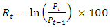
- Data Source, Transformation and Test Procedures This study used the daily and weekly all share index (ASI) of Nigeria stock market. The ASI spans January 30th, 2012 to December 8th, 2016, totaling 1,206 data points. The data were obtained from ww.africanfinancialmarkets.com. The daily ASI were transformed to daily stock returns, R𝑡, expressed as
 | (1) |
 is the return at time t, Pt is the price at time t; Pt-1 is the lagged price and
  is the natural logarithm.The Stochastic Volatility (SV) Model The widely used SV models can be described in its simplest form as follows.Let rt denote the mean corrected return observed at time t. As an example of return data rt, first consider pt which denotes, say, the Nigeria value of stock market at time t = 1, 2,…,n. Then mean corrected return, rt, can be computed as
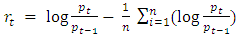 | (2) |
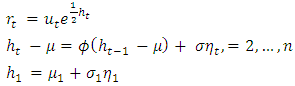 | (3) |
 and
and  are assumed to be a sequence of iid realizations from a distribution with mean zero and variance one. The parameters
  and
and  of the initial distribution are chosen (as a function of
  and
and  ) appropriately, so as make the process ht stationary when
  When
When  we set
  and
and  . Note that stationarity of the process ht implies stationarity of the process rt . In this work the
  and
and  are also assumed to be independent. However several extensions of the above model (3), are possible. For instance, [13], [14], [18] consider a SV model where
  and
and  are assumed to be correlated. To fixed the idea, let
  be the prior distribution of the unknown parameter
 or
or  in the unit root case), y = (y1, · · · ,yn) the observation vector, h = (h1, · · · , hn) the vector of the latent variables. Exact maximum likelihood methods are not possible because the likelihood
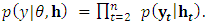
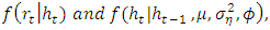
  does not have a closed-form expression. Bayesian methods overcome this difficulty by the data-augmentation strategy [26], namely, the parameter space is augmented from θ to (θ, h). By successive conditioning and assuming prior independence in θ, the joint prior density is
 | (4) |
 | (5) |
 | (6) |
 , one obtains the full conditional densities, i.e. the conditional density of a component of the vector of parameters given the other components and the observed data. Specifically, the conditional densities derive,
 | (7) |
 in model (2) respectively. Here
  is the vector of unobserved log-volatilities excluding the one at time t. The full conditional densities of
  are Normal and Inverse Gamma densities respectively.The full conditional density of
  is obtained as,
 | (8) |
 were the probability density functions of
  respectively.When we use a flat prior distribution, which is in the form of U(a,b) with b > 1 for the parameter
  the full conditional density of
  is given by,
 | (9) |
 with a constant mixing probability p, full conditional density of this parameter is given by,
 | (10) |
 are parameter to be estimated,
  are vector of unobserved log-volatilities and observed mean corrected return respectively,
 constant,
 and it is
  for
for  p = mixing probability.Testing the unit-root hypothesisIn order to test for the unit-root hypothesis
  versus
  Equation (3), extending the use of posterior credible interval approach in [14]. The test rejects the null hypothesis if the marginal posterior interval of 95% confidence level for
  does not include the unity. Rejection of the unit-root hypothesis implies that the volatility process is stationary and hence one can proceed with the application of inferential techniques in SV models that are developed under the stationarity assumption. On the other hand failure (if the null hypothesis is not rejected) to reject the null hypothesis implies that the volatility process is nonstationary and shocks to volatility have long-term effects. Therefore, this paper applied U (0, 1+c) type of prior density for
  at c = 0.0, 0.00001, 0.0001, 0.0002 and 0.001.
3. Results
- Descriptive Statistics Table 1 shows the descriptive statistics for All Share Index (ASI) and Returns to All Share Index (RASI). The notable difference in RASI is between its maximum 7.9% and minimum -4.4% values as well as when these values are compared with the mean value 0.018%, suggest some sort of variation in the series however, positive mean returns, indicate that, on the average, investors recorded gains more than loss during the sample period.
|
|

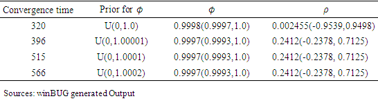
 imply that correlation between the error in the return and the error in the volatility may be ignorable, which were less than or equal to 0.2412 for different prior value. In this case, equation (3) is an overfit due to small value of correlation term. Parameter Estimates of Stock Volatility Clustering for Daily and Weekly Series The mean estimate of
  were found to be 0.7504 and 2.286 respectively for daily and weekly share price respectively, indicating volatility clustering in the series Table 3.
|
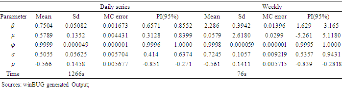
 does not only measured volatility clustering but it also indicated that news about volatility from the previous time periods has an explanatory power on current volatility. In contrast to the finding of [27] which recorded low value (
 = -0.03) using GARCH model implying volatility clustering takes less time to predict. A major economic implication of this finding is that investors of the Nigeria stock market though is volatile but increases or decreases of price movement is predictable over time.The Parameter
  estimated the mean of annualized returns which carried positive sign 0.5789 and 0.0579 for daily and weekly respectively, meaning that, annually on the average, investors recorded gain more than loss during the sample period. The small value of annualized return may be attributed to the economic crisis experience in the last decade. Again whenever markets were volatile return to investment tend to decrease sharply, this result suggested that investors should be updated or constantly monitor day to day transaction of stock markets. The mean estimate for parameter
  were 0.5505 and 0.7245 respectivetly for daily and weekly transaction. This measured variation of conditional returns distributed about the direction of price movement. The results of this findings revealed that the mean returns for investment were not normally distributed for the period of study. This recurrent fluctuation can only help investors’ to make decision for a short period of time. Leverage effect measured riskiness of a firm in relation to stock price movements. The model exhibited mean estimate of negative values for both series. The finding suggested that equal magnitude of bad news (negative shocks) have stronger impact on the volatility of stock index returns than good news (positive shocks). That is when stock prices are falling the value of equity decreases and the debt to equity ratio increases. Which cause firm to be more risky and induces a high future volatility.
4. Conclusions and Recommendations
- Stochastic volatility model could be used to test price movement in Nigerian stock market to make it better utilized by financial experts, econometrician and researcher. The study revealed there were significant variation in price movement of Nigerian stock market. There were significant presence of volatility clustered, leverage effects were exhibited by the mode. RecommendationIt is recommended that Stochastic Volatility (SV) models could be appropriate for real datasets such as stock market prices. This approach could be used to test the randomness in price movement of stock market. There were no significant difference between the means leverage effects for daily and weekly returns. Suggestion for Further StudiesFurther study should focus on selecting companies at random not in a generalized form in analyzing price movement in stock market. Companies should also be group into sectors (Oil and Gas, Banking sector, beverages, Insurance etc) before applying stochastic volatility model. Simulation should be carried out for different values of prior density for
 to test unit root based on posterior interval in order to reinforce or buttress the result obtained in this study.