1. Introduction

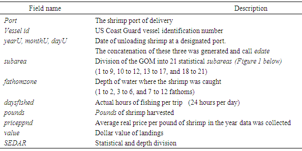
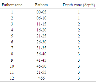
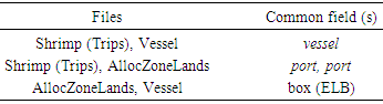
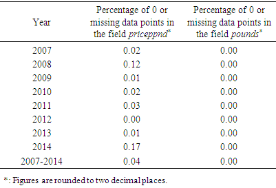
The primary objective of this research was to address the missing data points and handle those using proper statistical techniques. As an application, a general linear model (GLM) with a few covariates was developed and applied to the shrimp fishery data and estimated the fishing efforts (actual hours of fishing per trip) for the years 2007 through 2014. For estimating missing data points, multiple imputation method was selected and used. The method takes advantage of the Monte Carlo simulation along with statistical models in estimating missing data points [1]. Along with the objective mentioned above, the intention was also to show how imputation would produce compelling results in case of missing data points.

General linear models have been addressed by many authors such as [2], for example. There has been (and continue to be) advances made on this topic. The model has been extended to include stepwise regression, logistic regression, and general and generalized linear mixed models among others. There is no need to address this theory again here and it is assumed that the reader is familiar with this concept.

Due to the lack of familiarity and/or computational challenges, some researchers have relied on the ad-hoc approaches such as removing or replacing missing data points with the average of the existing points. These approaches may ultimately produce results far from the true values [3] and [4].

Consider a set of an ordered pairs of numbers (x, y) as (2, 6), (3, 7), (4, 8), (5, .), and (6, 10). Notice that the pair before the last is missing the y-component. The average of the existing y values is 7.75. On the contrary, one imputation method produces 9 for the missing value which is a much more reasonable value for the missing data point (given the pattern). It is a fact that replacing the missing value with the average of the existing y values relied only on the y values. The imputation method on the other hand, took advantage of an additional piece of information (that is, the x values) to produce an estimated value for the missing data point. We must use every piece of information available to us when trying to estimate a missing value (s).

Many research studies have addressed multiple imputation including [5-9]. Depending on the circumstances, for example, the pattern of missing data points, proper imputation models have been selected carefully and used here.

Data for the shrimp effort estimation come from dealers, port agent interviews, United States Coast Guard, (USCG) and Electronic Logbook (ELB) devices installed on vessels. The major data contributors to this research were the following three files: Shrimp data files (2007-2014), AllocZoneLands files (2007-2014), and the United States Coast Guard Vessel file. The Shrimp data file available from the National Marine Fisheries Service (NMFS) is based both upon landings as reported to NMFS port agents by dockside dealers and agent interviews with shrimpers who are in port [10]. The Shrimp data files included several fields of interest to this study. Table 1 gives the fields used in this research and the corresponding descriptions.

Table 1. Description of fields in the shrimp data file used in this research

The two additional files used in this research included the Alloczonelands and the Vessel files. The first contained Electronic Logbook Box number (ELB), edate, a combination of statistical subarea and fathomzone (zone), actual days fished (towdays), shrimp landings (landings), and port. The appropriate data points in this file were interviewed and recorded by the port agents at the designated ports. The second file called the Vessel file here was the US Coast Guard file containing vessel id number (vessel), ELB number, and the corresponding vessel lengths (length) among other pertaining information not used in this research.

To assist in the assignment of fishing locations, scientists have subdivided the U.S. Gulf of Mexico into 21 statistical subareas (Figure 1). Statistical subareas 1–9 represent areas off the west coast of Florida, 10–12 represent Alabama/Mississippi, 13–17 denote Louisiana, and 18–21 represent Texas. These subdivisions are used by the port agents and the state-trip-ticket system to assign the location of catches and fishing effort expended by the shrimp fleet on a trip-by-trip basis [11]. Each statistical subarea is further divided into five-fathom depth increments (Table 2). This table also includes fathomzones and the corresponding depth zones. The twenty-one statistical subareas are placed into four areas (1 through 4), and twelve-fathom zones are placed into three depths (1 through 3). Figures 1 and 2 display the 21 statistical subareas (1 through 21) and 12 area-depth combinations (Figure 3).

Table 2. Fathomzones (1-12), fathom, and corresponding depth zones (1-3) in the Gulf of Mexico

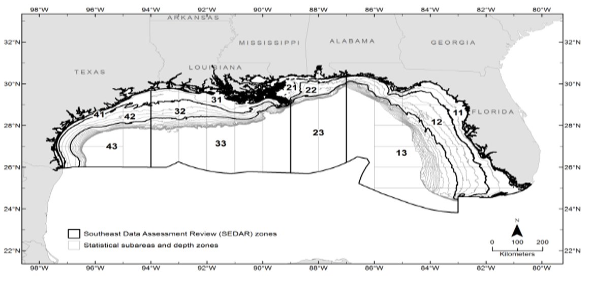
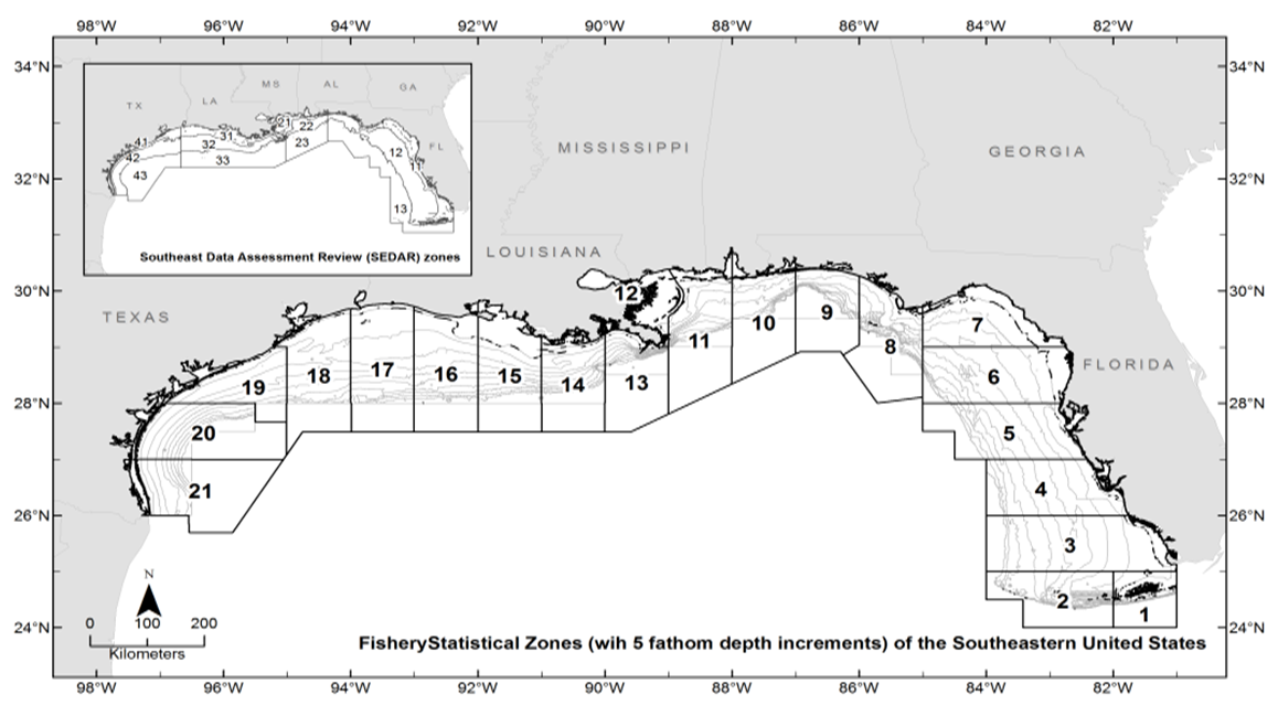Figure 1. The Gulf of Mexico is divided into twenty-one statistical subareas (1-21) as shown

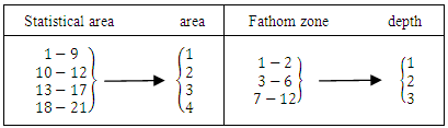Figure 2. Conversion of statistical subareas (1-21) and fathomzones (1-12) in the Gulf of Mexico to areas (1-4) and depths (1-3) respectively

Figure 3. Combination of areas (1-4) and depths (1-3) in the Gulf of Mexico called SEDAR cells

2. Method

2.1. Year-by-year

As described in [12], the following steps were taken to prepare the data for statistical analysis. First, for each year, the offshore data in the Shrimp data file was converted to “Trips” based on vessel id number (vessel), edate (edate), and port (port) along with the weighted average price per pound per trip (wavgppnd) and total pounds per trip (totlbs). In the next step, the three files Trips, AllocZoneLands, and Vessel were matched based on the common fields listed in Table 3 grouped by the zone field from the AllocZoneLands file to create the “Match” file. For the purpose of effort estimation later, the next step was to revisit the shrimp data file and convert it to “Trips” but this time grouped by the SEDAR field. In this research, the calendar year was also placed into three trimesters (January-April, May-August, and September-December).

Table 3. Common fields used in creating the Match file

2.2. Year as a Covariate

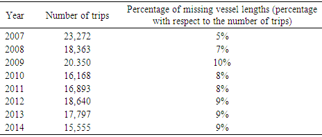
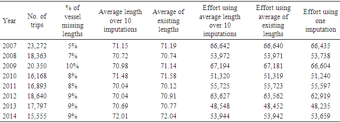
Here, the process again involved several steps. First, all the Shrimp files were merged to create one file consisting of 579,818 records (offshore data only). It was decided to impute the files for a few missing data points in the price per pound field prior to merging. The resulting file then was converted to “trips” based on vessel id number (vessel), edate (edate), and port (port). The new file called “Trips” had 82,856 records. At the same time, the weighted average price per pound using pounds as the weight (wavgppnd) and total pounds per trip (totlbs) were computed. Next, all the AllocZoneLands 2007-2014 files were merged creating a new file with 13,908 records. Similar to the case of year-by-year, the three files Trips (created above), new AllocZoneLands, (described above) and the Vessel file were matched based on the common field (s) listed in Table 3 and grouped by the field zone from the AllocZoneLands file. The resulting match file consisted of 61,232 records. For the purpose of effort estimation later, again the appended shrimp files described in the first step was converted to trips using Table 3 and grouped by the SEDAR field. The generated file consisted of 137,039 records (trips).

Real datasets often have missing data of one kind or another, an unpleasant reality that must be faced. The variable vessel length (length) was included in the model as a continuous predictor [12]. Due to the inclusion of length in this study, in the next step, the United States Coast Guard file (USCG) was used to locate as many vessel lengths as possible. Table 4 shows the number of trips generated and the percentage of missing lengths in the corresponding Trips files for each year.

Table 4. Number of trips and percentage of missing lengths in the Trips file (year-by-year) in the Shrimp file

The main contributor to the issue of missing data points was the vessel length (length). Reference [13] developed a simple linear regression between the vessel length and its horsepower. From a statistical perspective, this method is a good one as long as a satisfactory model can be established. In this research efforts in finding a simple or a multiple linear model between the known vessel lengths and variables such as pounds in the shrimp fisheries (2007-2014) did not produce a satisfactory result (R-Squared ranged from 0.03 to 0.08 with high absolute values of residuals). Therefore, the multiple imputation method was selected and used in estimating missing data points.

To estimate missing vessel length values throughout this article, multiple imputation was deployed. For comparison purposes only, an ad-hoc method (replacing missing lengths with the average of existing lengths) was also used in the study.

2.3. Handling Missing Data Points via Imputation

As mentioned above, in this article, the imputation method was selected as a mean for estimating the missing values. Using this method one can estimate a missing value statistically while considering the variability generated due to the selection of a value for the missing data point [1]. Since missing vessel length pattern could not be predicted from any other meaningful variable such as pounds, it was assumed that the missing pattern here was missing completely at random (MCAR), that is, missingness was not related to any factor, known or unknown [4]. In other words, 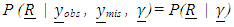where the vector represented the observed and missing vessel lengths (length), and represented the totlbs with all known values and a vector with elements 1 if a vessel length was missing and 0 otherwise. For a detailed definition of MCAR, the reader is referred to [14]. The 2008 data with moderate missing vessel lengths (7%) was selected and checked for the MCAR pattern. To confirm the MCAR pattern, Little’s test [15] was applied to the same data set producing χ² = 0.509 with p-value 0.476. Little’s test was also applied to the 2007 data for a confirmation of the pattern which produced χ² = 3.378 with p-value 0.066 (close to being significant using the threshold 0.05, but still non-significant). Therefore, it was assumed that the missing pattern was MCAR in all data sets used in this research. One could have also assumed the MAR condition (missing at random) as the missing pattern.

Imputation methods offers different models or mechanisms depending on the missing data pattern as discussed below. The reader is referred to an article by [16] for a comparison of different imputation methods.

2.4. Missing Data Pattern

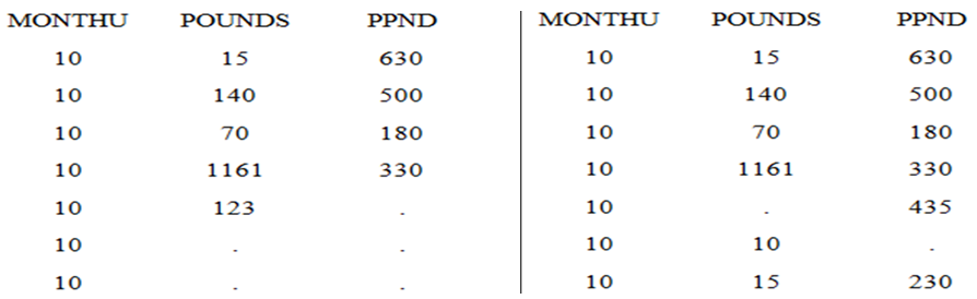
Before applying a multiple imputation to the data sets, it was important to identify the missing pattern(s) in the data set. In this paper, I identified two patterns: Monotone and Non-monotone (Arbitrary). As appeared in [17], a data set is said to have a monotone pattern if a triangle consisting of cells with missing value can be formed in the lower right corner (Figure 4a). In other words, if in the i^th row, Y_j is missing, all entries on this row following Y_j and subsequent columns below must also be missing. An arbitrary (non-monotone) pattern does not follow any specific missing pattern (Figure 4b).

Figure 4a. A monotone (.= missing value) & Figure 4b. An arbitrary pattern (.= missing value)

Monotone pattern offers flexibilities and some interesting features. Among those, it allows the user to impute missing values sequentially and to use regression model to impute variables. The restriction however is that the imputed variables must be continuous. To take advantage of monotone pattern, some researchers suggest that enough variables are imputed to make the data follow monotone patterns first [17].

For the 2007-2014 fishery data, the individual shrimp files contained some zero values the priceppnd (See Table 5).

Table 5. Percentage of missing or 0 data points in pounds or priceppnd field, years 2007-2014

The percentage of missing or 0 values in the priceppnd field in 2008 and 2014 were higher than the corresponding values in the other years. The corresponding values in the value field were also either missing or 0. In each case, the proper imputation method (monotone or arbitrary) was deployed and the missing points were filled via imputation with the imputed values.

2.5. Imputation Method

Multiple Imputation involves three distinct steps for each missing value.

Step I. The missing data are estimated m times (imputations) resulting in m complete data sets.

Step II. Each complete data set is analyzed by using standard statistical models such as regression.

Step III. The imputed values from the m complete data sets are averaged to get a value for the missing data point.

In what follows, I will explain each step very briefly.

Step I. In performing Step I, one needs to select a statistical model for the imputation. Depending on the missing patterns in the data set, several methods can be deployed.

2.5.1. Data Set with Monotone Pattern

A number of statistical models have been proposed when the data set has a monotone pattern and the variable is continuous. In the following, I briefly introduce a few of these models.

2.5.2. Propensity Score Method

As described in [17] and [18] in detail, the propensity score method is an imputation method applied to continuous variables when the data set has a monotone missing pattern. The propensity method does not use the correlations among variables, but focuses on the covariate information related to the missing value. It is not appropriate for analyses involving relationships among variables such as a regression analysis [19]. In addition, it should not be used when the predictors have missing values [20].

2.5.3. Discriminant Function Method

This model of imputation is the standard imputation method for categorical variables in a data set with a monotone missing pattern [17].

2.5.4. Logistic Regression Method for Monotone Missing Data

The logistic regression model is applied to categorical (binary) or ordinal variables and is considered an alternative to the discriminant function method [17].

2.5.5. Data Sets with Arbitrary Missing Pattern

For an arbitrary missing pattern and continuous variables, the well-known model is called Markov Chain Monte Carlo (MCMC). In this model, it is assumed that the joint distribution of missing and known values is normal [19]. Using the properties of Markov chains, the method constructs a chain repeatedly until the distribution of interest stabilizes. In the case of categorical or continuous variables, an alternative model is known as Fully Conditional Specification (FCS) can be deployed. In the FCS, it is assumed that we have the joint distribution for all variables [21]. For each imputed variable, the model involves two phases: The “fill-in” phase where the missing values are filled sequentially providing initial values for the second phase called “imputation.” In the latter phase, the missing values are imputed sequentially for a number of iterations called burn-in iterations.

Step II. In this step, each of m complete imputed data sets is analyzed separately using any statistical model. In general, most researchers use the same model as the one used in step I, but some also use different statistical models in this step [19].

Step III. Pooling m compete data sets

Assume that the variable Q with missing values is to be imputed m times. This produces m estimates for Q and its corresponding variance U, say, Q₁, Q₂,…, Q_m and U₁, U₂,…,U_m. As mentioned earlier, in Step II each imputation is analyzed using any standard statistical model. In Step III, the imputed values are averaged to get a value for the missing data point. More formally, the posterior distribution of Q is the average of complete data posterior distributions of Q for the complete data (Y_o,Y_m)

(3)

This is equivalent to the formula used by [22], page 476.

Then the sample mean and sample variance for the variable Q can be written as:

(4)

The within imputation variance is the variance where we do not account for the missing values and is found by averaging the variance estimates from each complete set of imputed data. Another quantity of interest is the variance between imputations (B), where

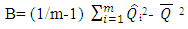(5)

This quantity measures the variation among imputed data sets. A small value for B indicates that the point estimates do not vary significantly from one imputation to the next. The average of B and T weighted by m imputations is called the total variance and is given by

(6)

A 100(1-α) % confidence interval for Q is given by

(7)

where,

(8)

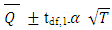
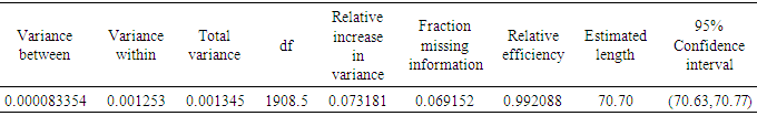
The pair determine the variability of The ratio indicates how much information is missing. That is, the fraction of missing information shown by δ. The relative efficiency of the estimate (RE) is defined as:

(9)

where m is the number of imputations and δ is the fraction of missing information [1]. For example, for an efficiency of 100%, an infinite number of imputations are needed. Table 6 helps guide the choice of value that should be used for m upon the selection of δ and the desired efficiency by the user. For other values not listed in the table, given the desired efficiency and δ, one can use the Goal Seek option provided in Microsoft Excel ⁽²⁾ to determine m.

Table 6. Some selected efficiency values for the number of imputations needed- m is the number of Imputations, δ fraction of missing information. Numbers in the body of the table represent desired efficiencies

2.6. The Model

2.6.1. Year-by-year

A GLM was developed to estimate shrimp effort in the Gulf of Mexico for the years 2007 through 2014. The vessel length (in feet) was used as a continuous predictor in the GLM and was implemented as a continuous variable [12]. The model considered for this study was a linear model where natural logarithm for variables with high variability was used.

(1)

or in a more convenient (matrix) form after converting to a logarithmic equation

(2)

where, is a column matrix of the natural logarithm of towdays, is an n x m matrix of repressors relating the vector of responses to and the vector of fixed and unknown parameters, the error term. The vector is assumed to be a normally, independently, identically distributed (iid) random variable with and In this model length is the vessel length, ln(totlbs) is the natural logarithm of total pounds of shrimp per trip, wavgppnd is the weighted average price per pound of shrimp per trip, area (a categorical variable with four levels), and depth and trimester are categorical variables with three levels. The response variable is towdays.

2.6.2. Year as a Predictor

The model considered here was similar to the case of year-by-year except year was added to the model as an additional covariate.

3. Analysis/Results

3.1. Year-by-year

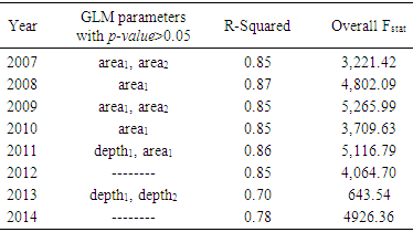
The model given in (1) was fitted to the corresponding Match file for each year and Table 7 shows the results of ANOVA where non-significant parameters and R-Squared values are listed (overall F_stat =16,832.2, p-value<0.0001). Subscripts following each categorical variable represent the levels of the corresponding variable. Due to a large number of parameters, only the non-significant ones (p-value>0.05) were included in the table 7.

Table 7. Non-significant GLM parameters and the R-Squared values (year-by-year). Subscripts represent the levels of the corresponding categorical variables

Table 8 displays the efforts generated via the GLM model for the years 2007 through 2014 depending on different ways of handling missing vessel length and Figure 5 is the display of the same. To preserve the integrity of the data sets, all calculations have been carried out to at least two decimal places and some rounded at the end to two decimal places (such as estimated vessel lengths).

Table 8. Effort generated via the GLM model for the years 2007 through 2014 year-by-year for different choices of missing vessel lengths using the monotone regression imputation method

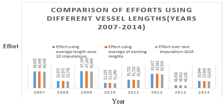Figure 5. Effort generated via GLM for the years 2007 through 2014 for different missing vessel length choices (one imputation, ten imputations or the average of existing vessel lengths) using the monotone regression imputation method

To assure the accuracy of the model given in (1), the empirical rule was used to check the necessary normality condition of the error term. Table 9 shows that the normality assumption of the error term was satisfied (empirical rule 1-sigam, 2-sigma, and 3-sigma).

Table 9. Observed and expected percentages using empirical rule (1-sigma, 2-sigma, and 3-sigma), in the case of year-by-year, for checking the normality assumption of the error term in the GLM

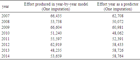
3.2. Year as a Predictor

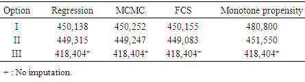
The model with year as a predictor was fitted to the related Match file created earlier. Out of several parameters in the model, the following were not significant (p-value>0.05): area₁, year₄, and year₆. The remaining parameters were significant with R-Squared=0.82 and F_stat = 16,832 and at p-value<0.0001. In order to measure the impact of using different imputation models used in this paper, efforts were generated using these models. Figure 6 displays the total effort estimates for a few imputation models defined in this paper.

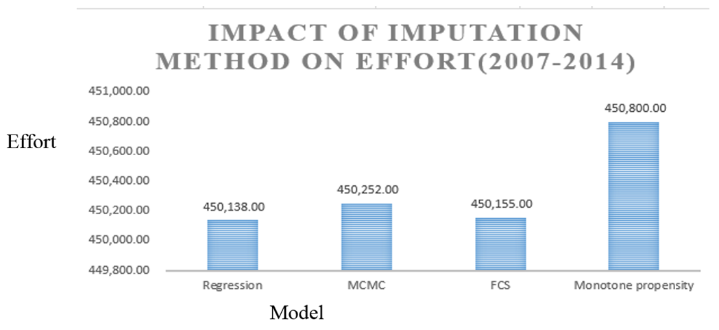Figure 6. Impact of imputation models on effort (year as a predictor): regression, MCMC, FCS, and monotone propensity

In order to compare the efforts produced using the year-by-year method, and those of year as a predictor, the total effort in the latter was broken into year-by-year. Table 10 displays the efforts produced in both cases. A comparison of year-by-year versus year as a predictor using a simple t-test under either equal or unequal variances showed that the two groups were not statistically different (t_stat = 0.33, t_crit = 2.14, and p-value = 0.74 under equal variances).

Table 10. Comparison of efforts produced year-by-year versus year as a predictor

Furthermore, the normality assumption of the error term in the GLM model was approximately satisfied. Table 11 shows the results of empirical rule applied to the residuals. The average effort over the period of eight years (2007-2014) in case of year-by-year was 57,303 and that of year as a predictor in the model was 56,267 for a difference of 1,036 towdays. In addition, in case of year as a predictor, the between variance over 10 imputations was 0.00009706 indicating that the imputed data points were estimated is a satisfactory manner. This was again due to a low percentage of vessels with missing lengths (8%).

Table 11. Observed and expected percentages using empirical rule (year as a predictor) for checking the normality assumption of the error term in the GLM

Again, in the case of year as a predictor, the between variance, the within variance, show that accounting for the missing values increased the variance by 7.3% as compared to performing the analysis without the missing values. A narrow confidence interval and very high relative efficiency were all indication of the fact that 10 imputations were sufficient to produce stable estimates (Table 12).

Table 12. Variance information associated with vessel length with m=10 imputations (year as a predictor)

For additional analysis, in the next step, three options were considered. The first option (I) was to impute all the missing or 0 values in the pounds, priceppnd fields, and the vessel length (length) in the combined shrimp data files where the year was used as a covariate. Effort generated in this option were displayed in Figure 6 and repeated again in Table 12. The second option (II) was to delete all the records in the combined shrimp data files where there were 0 or missing values in the pounds or priceppnd fields and estimated effort as in option I. The third was to remove all the records from the same data file where either pounds, priceppnd or length was 0 or missing and estimate effort again. The results are summarized in Table 13.

Table 13. Efforts generated under Options I, II, and III for the years 2007-2014

In the ANOVA table, the F_stat was significant (F_stat = 10.31, p-value = 0.0066) causing at the least, one of the effects to be significant. Analysis showed that there was no significant difference among the four imputation methods (F_stat = 1.25, p-value = 0.3731). However, the three options mentioned above differed significantly (F_stat = 23.91, p-value = 0.0014). Further, pairwise comparisons of Options I, II, and III placed Options I and II in one category and III in a separate category implying that the imputations of some data points in the pounds and priceppnd fields did not play a significant role in generating efforts.

4. Discussion

The main objective of this work was to introduce the imputation method to the fisheries data and use it to estimate the missing data points in the Gulf of Mexico shrimp data files. The issue of missing data points was briefly addressed in [12] where imputation was deployed in handling such points.

The contributor to the issue of missing data points was primarily the vessel length (length). One potential approach was to remove all the records with missing data points. This method has not been a popular approach among researchers as it reduces the sample size and results in a higher standard error (sample size n is in the denominator of the standard error formula). Alternatively, the missing data points could have been replaced with the average of the existing data points (Table 8 and Figure 5). For a comparison/contrast, this method was implemented here and the results were close to those of imputation. This was due to the low percentage of missing data points (Table 4). However, such substitution could have produced an estimate close to the actual value or something far away from it.

As mentioned earlier, efforts in finding a simple or a multiple linear model between the known vessel lengths and variables such as pounds in the shrimp fisheries (2007-2014) did not produce a satisfactory result (R-Squared ranged from 0.03 to 0.08). Such relation, if satisfactory, could have been used to estimate the missing data points. Regression models with low R-Squared and high residuals would likely produce unreliable estimates. Reference [23] in his article argued that “Though the correlation coefficient, 0.18, differed significantly (P< 0.05) from zero, the correlation was not a strong one, and it was not considered to be of practical significance.” It was ultimately decided to deploy the imputation method in handling the missing vessel length values and other missing data points. Following the imputation of missing data points, a general linear model was developed and used to estimate shrimp effort in the GOM for the years 2007 through 2014. In the following, I will discuss the year-by-year and year as a predictor results respectively.

4.1. Year-by-year

The analysis for the case where yearly data were analyzed separately suggested that the variable vessel length was statistically significant in the model estimating shrimp effort (p-value<0.0001) (See Table 6). Due to the low percentage of missing length, the estimated effort slightly changed when the model was run for different choices for the missing vessel lengths (Table 8 and Figure 5).

To compare the impact of the ad-hoc methods and imputation, the model was run for different years using these methods. The analysis showed that the methods considered here generated about the same total effort per year (Table 8, Figure 5). Due to a low rate of missing vessel lengths and the closeness of the generated efforts, it was unrealistic to compare the impacts of imputation and ad-hoc methods. However, as mentioned earlier, the imputation method takes advantage of many features and produces a more reliable estimate (s) as displayed via an example earlier.

4.2. Year as a Predictor

Similar to the case of year-by-year, the vessel length was a significant variable in the effort estimation model (t_stat = -35.56, p-value < 0.0001) and the missing vessel lengths did not play a significant role in the estimation process due to the low percentage of missing values (Table 4).

To measure the impact of different statistical imputation models on the shrimp effort estimation, four imputation models were deployed in the case of year as a predictor only (regression, MCMC, FCS, and monotone propensity). The monotone propensity model produced slightly higher towdays (662) over the period of eight years. As displayed in Table 12, Options I and II were placed in one category implying that the imputation of a few missing data points in either pounds or priceppnd fields did not play a significant role in the analysis.

5. Concluding Remarks

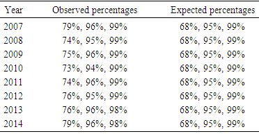
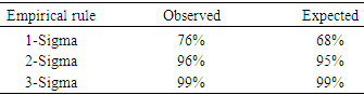
In this research, a few imputation models for handling missing vessel lengths were discussed. As mentioned earlier, replacing the missing vessel lengths with the average of the existing vessel lengths could produce estimates far from the true values. Of course, when there are few missing values, most (if not all) methods would do well. However, there is no guarantee that this is always the case. There is a likelihood of facing a large number of missing data points. Therefore, one needs to explore all the possibilities and select the most appropriate method by considering the tradeoffs between the complexity and accuracy. Although the generated efforts were very close, among several imputation models presented in this paper, due to its flexibility, a monotone imputation is preferred assuming that the necessary condition (s) is satisfied.

The analysis showed that the GLM model adequately represented the data sets in cases of year-by-year or year as a covariate. Reference [12] analyzed the same data using different statistical models. The model used in this article was much simpler involving fewer covariates. There is always a tradeoff between the complexity of the model and its accuracy or simplicity (Model parsimony). In this article, the main objective was to apply the imputation method to estimate missing data values in fisheries data.

In both cases of year-by-year and year as a covariate, the missing vessel lengths did not significantly change the total effort due to the low percentage of missing values. The necessary normality condition for the error term in the model was checked using the empirical rule. In either case, it was concluded that the proposed model represented the data adequately and estimated the total effort within the expected range. Furthermore, analysis with year as a predictor versus year-by-year produced similar results. In addition, the efforts produced under different imputation models were similar with one model producing a slightly higher estimate.

Although the application of the imputation method was limited to the shrimp data, it could be easily applied to other data sets. Missing data is common issue among data sets and this paper should be helpful in other areas of research.

ACKNOWLEDGEMENTS

The author would like to thank Mr. James Primrose of NMFS for providing the data sets for this research, Drs. Ryan Kitts-Jensen and Alex Chester of NMFS, and anonymous referees for their excellent editorial comments.

Disclaimer

The scientific results and conclusions, as well as any views or opinions expressed herein, are those of the author and do not necessarily reflect those of NOAA or the Department of Commerce.

1. The term SEDAR stands for South East Data, Assessment, and Review and is the cooperative process established in 2002 by which stock assessment projects are conducted in NOAA Fisheries' Southeast Region. SEDAR was initiated to improve planning and coordination of stock assessment activities and to improve the quality and reliability of assessments (http://sedarweb.org).

2. References to any software packages throughout this article do not imply the endorsement of the said products.