Peter Kirigiti Josephat1, Ahmed Ame2
1Department of Statistics, University of Dodoma, Dodoma, Tanzania
2Department of Management Sciences, University of Dodoma, Dodoma, Tanzania
Correspondence to: Peter Kirigiti Josephat, Department of Statistics, University of Dodoma, Dodoma, Tanzania.
| Email: |  |
Copyright © 2018 Scientific & Academic Publishing. All Rights Reserved.
This work is licensed under the Creative Commons Attribution International License (CC BY).
http://creativecommons.org/licenses/by/4.0/

Abstract
Logistic regression is widely used because it is a less restrictive than other techniques such as the discriminant analysis, multiple regression, and multiway frequency analysis. Because of it, many researchers do think that LR has no an assumption at all. The objective of this paper was to perform a complete LR assumptions testing and check whether the PS were improved. Agriculture data collected from 878 corn farmers were used. Six assumptions of LR were tested which included a sample size; expected cell frequencies; linearity in the logit; multicollinearity; outliers and influential cases; as well as the independence of residuals. A comparison of models was performed by comparing a model with the constant plus predictors with a model that had only the constant. Later, a model with only some predictors against the model with all predictors (full model) was compared to find out whether they were statistically significant. Findings have revealed that the two methods (significance of a variable testing and odds ratio) gave different variables to be included in the model. A statistically significant variable method gave better propensity scores than odds ratio method. An inclusion of only variables with an odds ratio >= 1 in the model, increased the dispersion of propensity scores when compared to the scores generated by the significant variables. Based on findings it is therefore recommended that all logistic regression assumptions, should be tested to ensure they hold in order to achieve better propensity scores for matching. Moreover, it is also recommended that variables which are to be included in the model should be based on significance testing.
Keywords:
Propensity Score Matching (PSM), Propensity Scores (PS), Weighted data, Un-weighted data, Logistic Regression (LR)
Cite this paper: Peter Kirigiti Josephat, Ahmed Ame, Effect of Testing Logistic Regression Assumptions on the Improvement of the Propensity Scores, International Journal of Statistics and Applications, Vol. 8 No. 1, 2018, pp. 9-17. doi: 10.5923/j.statistics.20180801.02.
1. Introduction
Logistic regression (LR) is widely used as a multivariate statistical method for analysis of data of one level nominal (dichotomous) dependent variable against predictors [11]. The method is increasingly applied in different specialization such as health, social sciences, educational research, etc. LR was introduced in the 1970s to overcome the limitations of ordinary least squares (OLS) in analyzing dichotomous outcomes [10].LR is widely used because it is more flexible (less restrictive) than other techniques such as the discriminant analysis, multiple regression and multiway frequency analysis [15]. It is flexible in the sense that, it does not require data to be normally distributed with an equal variance and covariance for all variables. LR makes no assumptions on the distribution of the explanatory data contrasting to the discriminant analysis. These methods are not different in their functional forms. Nonetheless, LR is appropriate and better in all other situations except when normality assumptions are fulfilled. Moreover, it fits well with many types of distribution [11].Propensity Scores are the estimated probability of the unit of analysis receiving the treatment given by the pre-treatment characteristics [16]. It is a probability of a unit which receives the treatment, given a set of the observed variables [3]. PS are used to compare (matching) treatment units in observational studies in order to determine the causal effects. During a PS matching, statistical techniques are used to assess effects of treatment by comparing the treated and untreated units. The interest of matching is to find if PS are the same for the control and treatment units.PS are mean generated based on certain variables. These variables are selected in such a way that, they are not affected by the treatment. They are used when treatment assignment is not random, as well as to reduce the bias in estimating the treatment effects and allow investigators to reduce the likelihood of confounding when analyzing nonrandomized observational data [6]. They are also used to estimate the causal impact of a treatment or intervention when units are not randomly assigned [7]. There are at least four PS methods which are used to remove the effects of confounding when establishing a causal effect of a non-experimental. These include the propensity score matching (PSM), stratification (or sub-classification) on the propensity score, inverse probability of treatment weighting (IPTW) by using the propensity score, and covariate adjustment by using the propensity score [1].PS typically are computed by using a logistic regression (LR) [3]. LR has been widely used as a statistical modeling in generating PS, especially, when dependent variable has a binary response. It is used in model fitting in order to examine the relationship between the dichotomous dependent variable and independent variables [12].Despite the fact that, LR does not assume normality, a constant variance of residuals, no linear relationship between the dependent and independent variables, many researchers do think that LR has no assumptions at all. Logistic regression assumptions on multivariate normality and linearity among predictors are tested as suggested [15]. These assumptions, are tested because a linear combination of predictors is used to form exponent. Moreover, continuous independent variables (IVs) are linear to logit of the dependent variable. If these assumptions are met, the power of the model is enhanced.The objective of this paper was to perform a complete LR assumptions testing and check whether PS are improved. In addition to the methodological contribution on PS estimation, this paper provides knowledge for researchers on LR assumptions procedures. Most researchers, jump into data analysis without putting much attention in model assumptions testing.
2. Procedures and Methods
This section discusses procedures and methods used to assess the variables to be included in the LR model, through testing its assumptions. Agriculture data collected from 878 corn farmers were used. Six assumptions of LR were tested which include: a sample size; expected cell frequencies; linearity in the logit; multicollinearity; outliers and influential cases; as well independence of residuals.Thirteen predictors were used to generate odds of being participated in agriculture intervention (dependent variable). Farmers participating in agriculture intervention were coded 1 while farmers not participating were coded 0. Predictor variables included: sex, age, type of farmer, marital status, education, household size, land owned, distance to corn farm, district headquarters, distance to tarmac road, climatic condition (weather), soil type and membership in other Participatory Farmer Groups (PFG).After testing the LR assumptions, a comparison of models was performed by comparing the model with the constant plus predictors, with the model that had only the constant. Later, the model with only some predictors against the model with all predictors (full model) was compared to find out whether they were statistically significant.
3. Results and Discussions
3.1. Testing Assumptions of Logistic Regression Model
This section assesses the requirements needed to be fulfilled before running a logistic regression model.
3.1.1. Sample Size
A logistic regression analysis, requires large samples be compared to a linear regression analysis because the Maximum Likelihood (ML) coefficients are large sample estimates. ML is efficient for large samples because it involves all moments [13]. In their experiment, which found out that, by committing type I errors does not change substantially, as the sample size decreases but the risk of committing type II errors is increased dramatically when the sample size is small and the number of regressors increases [5]. There are rules of thumb which are used to determine the number of cases necessary for testing the correlation and testing the individual predictors in regression [15]. One of the rules of thumb is that  + {8 x the number of Independent Variables, (IVs)} is the required sample size if the interest is to test the multiple correlations. If the study was to use a multiple regression analysis, then it required a sample size of
  (note IVs = 13). If the interest was to test the individual predictors, then
  would be required. For this case, a sample size of 154 could suffice both the overall correlation and the individual IV. More complex for the rules of thumb that consider the effects size are discussed by [4]. For a logistic regression analysis generally a minimum of 50 cases per predictor is recommended. Since thirteen variables were considered to determine the number of farmers to participate in agriculture intervention, a sample size of at least 650 cases was required. That is 13 x 50 = 650. The sample size of the study was 878 which indicated that, the ratio of cases to variables was highly satisfactory.
3.1.2. Expected Cell Frequencies
In order to use the goodness of fit test of the model, it is recommended that the expected frequencies should not be too small [15]. The expected cell frequencies are values which represent the frequencies expected to be found in cells if the null hypothesis was true. They are calculated from the marginal totals. Equation (1) is a formula to calculate the expected cell frequencies. | (1) |
where  is the expected frequency for the cell in the
  row and the
  column,
  is the total number of subjects in the
  row,
row,  is the total number of subjects in the
  column, and
  is the total number of subjects.The expected frequencies need to be > 5 and no more than 20% to count less than five. If this assumption is violated, the statistics chi-square value tends to be large with more frequency. This leads to an overestimation of the statistical significance, especially for small data. Thus, it is also very crucial to evaluate the expected cell frequencies. All pairs of all categorical variables including the outcomes were evaluated. The variables include sex, type of farmer, marital status, weather, soil type, member of other PFG and the experimental group.In examining the expected frequencies of sex and type of farmers, the odds ratio was used because the variables are nominal with only two possible responses each, (male/female and small/medium scale). Pairs of these two variables had no any cell with the expected count less than 5. The odds ratio for sex was 1.341 which showed that a male had 1.341 times the odds of being a small-scale farmer than a female. The relative risk of the farmer to be a small scale farmer was 1.004 while that of being a medium scale farmer was 0.749.The expected frequencies of sex and marital status showed that none of the cells had the expected count less than 5. The minimum expected count was 8.99 while the expected frequencies of sex and climatic condition showed, 2 cells had expected the count less than 5, which constituted 14.3%. Although the percentage was lower than 20%, the two cells with less than 5 counts, were found in the category of the average rainfall and sunshine. In order to improve the expected frequencies, the category was merged with sufficient rainfall. By so doing, none of the cells had expected frequencies of less than 5 as the minimum count was 12.85.The pair of sex and soil type generated 2 cells which counted less than 5 which formed 20%. Saline and peaty soil type were merged to get rid of the problem. This resulted in 0 (0%) cells which had counts less than 5. The variables sex and members in other PFG had also 0 (0%) cells, which counted the expected frequency with less than 5. The expected cell frequencies for sex and participating in agriculture intervention were as required. The pair of the type of farmers and marital status generated 4 cells (40.0%) with an expected count less than 5. In order to achieve the required expected cell frequencies, the separated and divorced marital categories were merged. The same applies to widows and singles. Despite merging of these categories, 33% of the expected frequencies counted less than 5. Furthermore, after merging the marital status categories to have only two (married and not married), the expected cell frequencies remained high at 25%. When evaluated with other variables, it was found out that, the variable had expected the cell frequencies higher than 20%.The evaluation of the expected cell frequencies of marital status and climatic condition showed that 22 (62.9%) had counts less than 5, while marital status and soil type were at 40%. The control was done by re-categorizing variable marital status to two categories which were married and not married. Thereafter the expected cell frequencies between marital status and the variables climatic condition, soil type, membership of the other PFG and participation of farmers to the intervention were 8.3%, 12.5%, 0% and 0% respectively.For the pair of the two variables climatic condition and soil type, 5 cells (20.8%) had expected to count less than 5. To improve the frequency of the cell, peaty, clay and saline categories were merged and thus, none of the cell frequency counted less than 5. The expected cells frequencies for the pair of the climatic condition and the member of the other PFG variables and that of the climatic condition and experimental group each counted 0% for less than 5. The expected cell frequencies for the soil type against the members of the other PFG and experimental group counted 0% for less than 5. The variables members of the other PFG and participation in intervention counted 0% for less than 5 too.
3.1.3. Linearity in the Logit
Although there are no assumptions about the linear relationship among predictors, logistic regression assumes a linear relationship between the continuous predictors and the logit transform of the dependent variables (equation 2). | (2) |
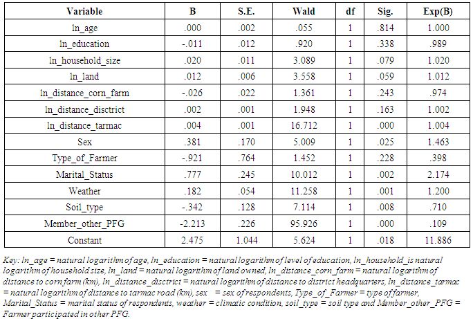
The assumption is tested by adding new variables (interactions between each continuous predictor and its natural logarithms), against the experimental group (dependent variable). This transformation is called Box-Tidwell [variable*ln x (variable)]. From Table 1, it can be observed that the additional variable ln_distance_tarmac is statistically significant. An assumption is violated which suggest that the variable requires improvement.Table 1. Logistic Regression Output for Interaction between Predictors and their Natural Logarithm
 |
| |
|
In order to improve results, the variable “type of farmer” which failed to count less than 20% of the expected cell frequencies of less than five was dropped. The variable distance to tarmac road was also investigated and found that, there were five mild outliers (Figure 1).  | Figure 1. Box Plot for Distance to Tarmac Road |
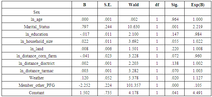
After running the logistic regression, results showed that the variable ln_distance_tarmac was no longer statistically significant (p = .072) which implied that, the assumption of linearity in the logit was not violated (Table 2). This being the case, there was no reason for transforming the variable.Table 2. Logistic Regression Output for the Interaction between Predictors and Their ln after Modifications
 |
| |
|
3.1.4. Multicollinearity
Logistic regression is a very sensitive to extreme high correlation among IVs. The standard errors for the “B” coefficients were examined, to test for multicollinearity. From Table 3, it can be found out that, there was no evidence of multicollinearity because none of the independent variables had a standard error larger than 2.0. Table 3. Standard Errors for B Coefficients
 |
| |
|
3.1.5. Outliers and Influential Cases
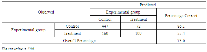
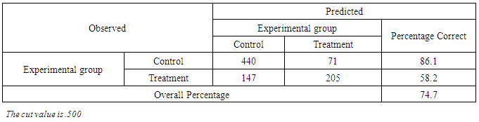
By excluding the outliers from the analysis substantially, an accuracy of the model is improved. A poor fit of the model occurs also when the category of outcome shows a high probability of being in another category. An outlier is checked by examining residuals. Residuals for each case are computed and then standardized, to assist in the evaluation of the fit of the model to each case. Influential cases are identified through Cook’s distances test as recommended [15].Outliers were checked by comparing the accuracy rates of the model that included outliers and the one which excluded the outliers. After running the residuals, it was revealed that there were eight outliers which had standardized residuals of ≤ -2.58. Furthermore, it showed that there were seven outliers with a large positive standardized residuals (≥ 2.58). For the case of Cook’s value, the output showed that no case had a value distance ≥ 1. This indicated that there were no any influential cases.Since the outliers were found, the logistic regression model which excluded outliers was performed. A classification accuracy rate of the model which included outliers was 73.6% (Table 4) while the rate of the model which excluded outliers was 74.7% (Table 5).Table 4. Classification Accuracy Rate of the Baseline model
 |
| |
|
Table 5. Classification Accuracy Rate of the Revised Model
 |
| |
|
The classification accuracy of the model which included all cases (baseline model) was 1.1% less than the classification accuracy for the model which excluded 15 cases found to be outliers. Since the accuracy rate of the revised model was less than 2% more accurate, logistic regression computations were based on the baseline model.
3.1.6. Independence of Residuals
Independence of errors was tested to observe if the responses of different cases were independent of each other. If errors are not independent it means that logistic regression produces an overdispersion (great variability) effects. Because of this, it was necessary for the assumption to be tested.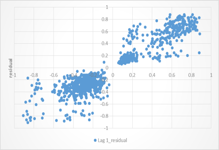 | Figure 2. Residual Lag Plot |
Independence of errors in logistic regression assumes a between-subjects design. The plot of residual and lag of residual in Figure 2 showed that there was a slight pattern of errors indicating that, a variance was non-random. The severity of the problem of an over-dispersion was assessed basing on Pearson and Deviance statistics. A Pearson value was found out to be 923.544 while Deviance statistic was 886.319. Coefficient of variation (CV) of the two values was found to be 0.029 obtained from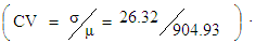 Since
Since  , it indicates that discrepancy of Pearson and Deviance was low (923.544 - 886.319 = 37.225). This suggests that an over-dispersion was not a problem.
3.2. Assessment of Contribution of Variables in the Model
This section discusses the importance of variables to the model. Two inferential tests were used: the tests of a model and the individual predictors.
3.2.1. Goodness of Fit of Models
At first, the independent variables were tested by comparing with the constant only model with the full model (constant and all variables), to find out whether they contributed to the prediction of the outcome. The two models were compared through -2log-likelihoods (equations 8 and 9), Akaike Information Criterion (AIC) (equation 10) and Chi Square. All these tests are used to find out which model approximate the reality given to the set of data. The idea of comparing models was to find out the model with a minimal loss of information than others. Statistical significance difference between the models indicates the relationship between the predictors and the outcome [15].Log-likelihood is calculated basing on summing the probabilities associated with the predicted and the actual outcomes for each case: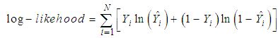 | (3) |
Log-likelihood is multiplied by -2 in order to have a statistic that is distributed as chi-square. 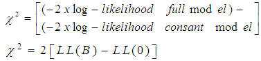 | (4) |
AIC originated from Kullback-Leibler Information (KLI). It represents the information lost when the reality is approximated [8]. Through AIC, the relationship between the Maximum Likelihood and KLI information is established which is defined as; | (5) |
Whereby K, is the number of estimated parameters included in the model (variables and constant). The output showed that AIC value for the baseline model (a model which contained only a constant) was 1,189.846 while for the full model (model contained constant and variables) was 923.125. Since the full model had a lower value than the constant model, there were indications that, the full model was a better fit. -2log-likelihoods values were found to be 1187.846 for the baseline model when compared to 885.125 for the full model. Like AIC, the lower value indicated a model fit. There were indications that, a full model fitted data well when compared to the baseline model.Furthermore, it was found out that, the baseline model was accurate by 59.1%. This indicated that by nature the model had a predictive power. Omnibus tests of the model coefficients showed further that, the chi-square was significant;  at 0.05. This is an indication that, there was a significant difference between the log-likelihoods between the baseline model and the new model (full model). Because the difference was significant, it implied that the new model was improved as it had significantly reduced -2LL compared to the baseline model. Variance in the outcome variable is more explained in the new model. Nagelkerke
  suggests that the model explains about 39% of the variation in the outcome. The Hosmer-Lemeshow statistic, indicates a good fit because
 (A significant test indicates that the model is not a good fit and a non-significant test indicates a good fit). The tests show that the new model adequately fits the data. The classification rate accuracy of the new model was improved as it stood at 73.6% when compared to 59.1% of the baseline model.
3.2.2. Tests of Individual Variables
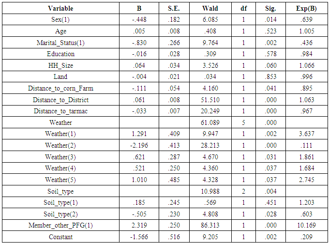
In order for any model to be lively, apart from other things, it requires to contain variables which have enough contribution. Besides to this, outcomes generated will be of doubt. There are several ways of testing whether the variables included in the model have required contribution. One of the most common methods of testing variables to be included in the model is through the p-value. Despite of being widely used, p-values suffer several shortcomings. They simply give a cut-off beyond which the conclusion is reached whether to reject a null hypothesis or not. [2] argue that non-significant results do not imply that there is no effect. Statistical significant results also do not necessarily imply that the effect is physical. The importance of variables in the model is determined by size of the effects and not statistical significance. Effects size also known as the standardized mean difference, are measured in various ways such as an absolute risk reduction, relative risk reduction, relative risk, odds ratio [2]. An odds ratio is used for binary or categorical outcomes [9]. The examination of variables in the model was done by basing on the p-values and odds ratio. Thereafter, propensity scores were generated to observe if there was any significant difference. From Table 6, it can be seen that, out of the twelve variables included in the model, seven were significant since their p-values were less than 0.05. These are sex (p = 0.002), marital status (p=0.000), household size (p=0.029), distance to corn farm (p=0.001), distance to district (p=0.000), distance to tarmac (p=0.023) and participation in other PFG (p=0.000). This statistical significance of the coefficients was based on Wald test, that is,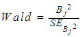 | (6) |
Odds ratio (OR) shows that, out of the twelve variables, seven had odds ratio values greater than or equal to 1 which indicated that, their contribution to the model was positive. The variables are sex (OR =1.672), Age (OR = 1.000), marital status (OR = 2.557), household size (OR = 1.073), land (OR = 1.020), distance to district (OR = 1.023) and weather (OR = 1.072).Results show that, it is not necessary for a variable to be significant and at the same time having an odd ratio of 1 or above. Only four variables were both significant and had positive odds ratio namely; sex, marital status, household size and distance to a district. The significant variables are bolded as presented in Table 6.Table 6. Variables in the Model
 |
| |
|
However, the propensity scores of the three models were examined to observe the differences (Table 7). The first model contained thirteen variables, while the second contained only those variables which were significant. Furthermore, the third model contained variables with odds ratio ≥ 1. Propensity scores were compared based on control and the treatment group by using the independent t test. Before comparing scores of the control and treatment groups, a balance of matching was examined through univariate and multivariate balance statistics. A matching balance is checked for a model containing significant variables and the variables with positive odds. For a model which involves significant variables only, an overall chi square balance test, is not significant . Multivariate imbalance measure
  for the unmatched solution (before matching), was 0.936 while after matching was 0.920. Both Chi square test and multivariate imbalances showed that, there were no imbalances after matching. Multivariate imbalance indicated that, there was no imbalance because the value for matched sample was small (0.920) than unmatched sample (0.936).
 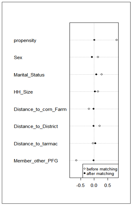 | Figure 3. Standardized Mean Differences based on Significant Variables |
The standardized mean difference shows that, all covariates are balanced as  . The magnitude of the standardized mean differences before and after matching is presented in Figure 3 which shows that, the propensity scores of the variables after matching are very close to the middle column (dashed line) compared to propensity scores before matching. This indicates that, there is an improvement of the magnitude of the mean difference. After ensuring that the scores were balanced, an independent t test was performed to assess the difference between the scores of control and treatments (Table 7) after the six variables which were not significant and then were dropped from the logistic model. For the model with variables which achieved the odds ratio of 1 and above, the overall chi square balance test was not significant
 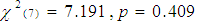 . Multivariate Imbalance Measure
  for the unmatched solution (before matching) was 0.976 while after matching was 0.981. On the other hand, the chi square test shows that, there was no imbalances after matching, multivariate imbalance test indicated that, there was imbalance because the value had increased from 0.976 to 0.981. Unbalanced covariates test shows further that, no covariate exhibit a large an imbalance i.e.
  . The magnitude of the standardized mean differences before and after matching is presented in Figure 4 which shows that, there was no improvement of the magnitude of the mean difference rather, the dispersion of propensity scores to the dashed column was large when compared to Figure 3. All tests were not holding to ensure that, there were no imbalances of scores. Despite of this, the difference of scores between the control and treatment were computed.
 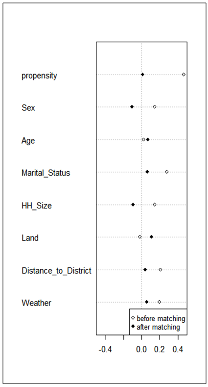 | Figure 4. Standardized Mean Differences based on Odds Ratio |
The differences in the mean of propensity scores for all cases were not significant as shown in Table 7. By observing at the standard errors, it can be found out that, the last two models had small errors when compared to the first model which showed that, the two models produced more statistical accurate estimates. Table 7. Comparison of Propensity Score Matching
 |
| |
|
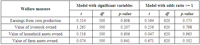
The study was more interested to observe to what extent the propensity score of the two new models affected results on the welfare of farmers (Table 8). Welfare is used to test performance of the models. The study showed that, neither of the factors was significant. Since the t values were positive, it indicated that there was an increase of earning from corn production, the value of livestock, households assets and farm assets of farmers participated in the agriculture intervention when compared to whom did not. Nonetheless, the increase is not significant. Table 8. Welfare Assessment Basing on New Models
 |
| |
|
4. Conclusions
Following the above discussions, it is revealed that, by reducing or merging some categories of the variable expected cell frequencies improved. Another finding is that, when a variable with a high percentage of the expected cell frequencies is dropped, the result is further improved.It is not necessary for the variable to be significant and at the same time, having an odds ratio of 1 or above. [14] says that the presence of a positive OR for an outcome given to a particular exposure does not necessarily indicate that, the association is statistically significant.If a variable exhibits the extreme values (outlier) and is excluded in the analysis, the accuracy of the model is substantially improved. Furthermore, another discovery is that the two methods (significance of a variable testing and odds ratio) give different variables to be included in the model. The significance of the variable method gives better propensity scores than odds ratio method. The inclusion of the only variables with odds ratio >= 1 in the model, increases the dispersion of propensity scores compared to the scores generated by the significant variables.Based on the findings it is therefore recommended that;(i) All logistic regression assumptions, should be tested to ensure they hold in order to achieve a better propensity scores for matching. (ii) Because the model which contained variables with odds ratio >= 1 only gave a poor propensity scores than the model contained significant variables only, it is recommended that variables to be included in the model should be based on the significance testing.
References
| [1] | Austin, P. C. (2011), “A Tutorial and Case Study in Propensity Score Analysis: An Application to Estimating the Effect of In-Hospital Smoking Cessation Counseling on Mortality”, Multivariate Behavioral Research, 46:119–151. |
| [2] | Davies, H. T. and Crombie, I. K. (2009), “What are Confidence Intervals and P-Values?”, [http://www.medicine.ox.ac.uk/bandolier/painres/download/whatis/What_are_Conf_Inter.pdf], site visited on 25/5/2015. |
| [3] | Domingue, B. and Briggs, D. C. (2009), Using Linear Regression and Propensity Score Matching to Estimate the Effect of Coaching on the SAT, Unpublished research report, University of Colorado. |
| [4] | Green, S. B. (1991), “How Many Subjects Does it Take to do a Regression Analysis?” Multivariate Behavioural Research, 26, 449 – 510. |
| [5] | Hart, R. A. and Clark, D. H. (1999), “Does Size Matter? Exploring the Small Sample Properties of Maximum Likelihood Estimation” in Proceedings from the Annual Meeting of the Midwest Political Science Association; Chicago IL. April. |
| [6] | Haukoos, J. S. and Lewis, R. J. (2015). The Propensity Score. JAMA, Vol. 314(15): 1637 – 1638. |
| [7] | Keller, B. and Tipton, E. (2016). Propensity Score Analysis in R: A Software Review. Journal of Educational and Behavioral Statistics, Vol. 41 (3): 326 – 348. |
| [8] | Kullback, S. and Leibler, R. A. (1951), “On Information and Sufficiency”, Annals of Mathematical Statistics 22:79-86. |
| [9] | Nandy, K. (2012), “Understanding and Quantifying Effect Sizes”, [http://nursing.ucla.edu/workfiles/research/Effect%20Size%204-9-2012.pdf], site visited on 25/5/2015. |
| [10] | Peng, C. J. and So, T. H. (2002), “Logistic Regression Analysis and Reporting: A Primer”, Understanding Statistics I (1), 31 – 70. |
| [11] | Pohar, M., Blas, M. and Turk, S. (2004), “Comparison of Logistic Regression and Linear Discriminant Analysis: A Simulation Study”, Metodološki zvezki, Vol. 1, No. 1, 143-161. |
| [12] | Sarkar, S. K., Midi, H. and I. A. H. M. R. (2009), “Binary Response Model of Desire for Children in Bangladesh”, European Journal of Social Sciences, 10(3). |
| [13] | Schoonbroodt, A. (2004), “Small Sample Bias Using Maximum Likelihood versus Moments: The Case of a Simple Search Model of the Labor Market. University of Minnesota”, [http://www.economics.soton.ac.uk/staff/alicesch/Research/smallsammlmomjae.pdf], site visited 05/05/2015. |
| [14] | Szumilas, M. (2010), “Explaining Odds Ratios”, Journal of the Canadian Academy of Child and Adolescent, 19(3): 227–229. |
| [15] | Tabachnick B. G. and Fidell, L. S. (2007), Using Multivariate Statistics: Fifth Edition, Person Education Inc. |
| [16] | Trojano, M., Pellegrini, F., Paolicelli, D., Fuiani, A. and Di Renzo, V. (2009), “Observational Studies: Propensity Score Analysis of Non-randomized Data”, The International MS Journal, 16, 90–97. |

 Abstract
 Reference
 Full-Text PDF
 Full-text HTML