1. Background to the Study

Apparent temperature allows for the quantitative assessment of heat stress and is used to determine the limit of heat exposure in order to prevent heat related illnesses. The Heat Index was originally developed by Steadman (2011) as an assessment for sultriness, but commonly referred to as the apparent temperature. Parameters involved in determining apparent temperature are water vapor pressure, surface area of skin, significant diameter of a human, clothing, core temperature, activity, effective wind speed, clothing resistance to heat transfer, radiation to and from the skin’s surface, sweating rate, ventilation rate, skin resistance to heat transfer, and surface resistance to moisture transfer. The heat index is the measure of how hot it really feels when relative humidity is factored with the actual air temperature (Rothfusz, 1990; Mendelsohn, 2003; Epstein, 2006; Robert, et al. 2010; Anderson et al. 2013; NOAA, 2013; Qu, et al. 2016). In estimation of ARIMA (p,d,q) model the researchers often peg the value of d as an integer value most especially between 0 and 2, however in estimating d in practice it is not always an integer value there are often at times that the value of d lies between -0.5 and 0.5. Many time series exhibit too much long range dependence to be classified as either I(0) or I(1) but do not belong to either of them. In the recent, majority of these long range dependence models are often called long memory models are normally taken care of by the Autoregressive Fractional Integrated Moving Average (ARFIMA) model. The series that exhibits long memory process has autocorrelation function that damps hyperbolically more slowly than the geometric damping exhibited by “short memory” autoregressive moving-average, ARMA(p,q) process, which is predictable at long horizons(Granger, et al. 1980; Hosking, 1981; Ding, et al. 1993; Taqqu, et al. 1995; Baillie, 2006; Robinson, 2003; Agostinelli, et al. 2003; Larranga, 2002; Nesrin, 2006; Haldrup, et al 2007; Baum, 2013; Contreras-Reyes, et al. 2013). Prior to this investigation on long memory of heat index in BIRNIN KEBBI metropolis, there have been previous studies involving heat in other fields such as Agric, Engineering, Physics, Chemistry or Biology in KEBBI State but little or no enquiry has been carried out on long memory effect of apparent temperature in KEBBI using time series approach. Over the years, there tends to be a severe heat during a particular period each year in the investigated area. This means we have higher values of heat index at a particular point in time every year. The research aims at investigating the long range dependency characteristics of apparent temperature in BIRNIN KEBBI metropolis with a view to determining: (i) the autocorrelation pattern for the long range dependency of the data points for the research; (ii) fractional value of d for the data points; and (iii) interpret the long memory characteristics.

2. Methodology

We adopted time series methodology to long memory characteristic of apparent temperature in BIRNIN KEBBI metropolis. It deals with hourly data of heat index collected over a period of two years from 2013 to 2014, and the set of data would be subjected to statistical testing procedures to confirm if the data are truly long memory, integrated, or stationary processes. It is expected to add to the existing literature on long memory behavior in heat index and will tend to help the metrology or practitioners in field of hydrology or dendrology. The data are secondary and are collected from Energy Research center BIRNIN KEBBI.

2.1. ARMA Process

An autoregressive moving average (ARMA) process consists of both autoregressive and moving average terms. If the process has terms from both an AR(p) and MA(q) process, then the process is called ARMA(p, q) and can be expressed as:

(1)

where is a white noise distribution term, so that for all t, and are serially uncorrelated. All ARMA models are stationary. If an observed time series is non-stationary (e.g. upward trend), it must be converted to stationary time series (e.g. by differencing) (Anderson, et al 1979; Pelgrin, 2011).

2.2. ARFIMA Process

ARFIMA process allows for long memory series to be fractionally integrated. The general form of fractional ARMA model or the ARFIMA (p,d,q) model is:

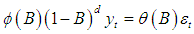(2)

Where d denotes non-integer fractional differencing parameter, is the dependent variable at time t, is distributed normally with mean 0 and variance , and represents AR and MA components respectively; and have no common roots, B is the backward shift operator and is the fractional differencing operator given by the binomial expansion: for large j is and is a white noise sequence with zero mean and Innovation variance . The properties of an ARFIMA process area bridged in the following theorem. Let be an ARFIMA (p,d,q) process then:

(a) is stationary and invertible if and all the root of lie outside the unit circle .

(b) is non-stationary if and all the root of lie outside the unit circle.

(c) if , the autocovariance of , as ; where B is a function of d.

The autocovariance function of ARFIMA process decay hyperbolically to zero as in contrast to the faster geometric decay of a stationary ARMA process.

2.3. Portmanteau Test

It is a test used for investigating the presence of autocorrelation in time series, number of lags µ and h are predetermined.

Hypothesis

(all the lags correlating are zero)

i.e for at least one i=1,…..h is tested i.e at least one lag with non zero correlation.

Test Statistic

where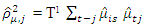

3. Analysis of Data and Results

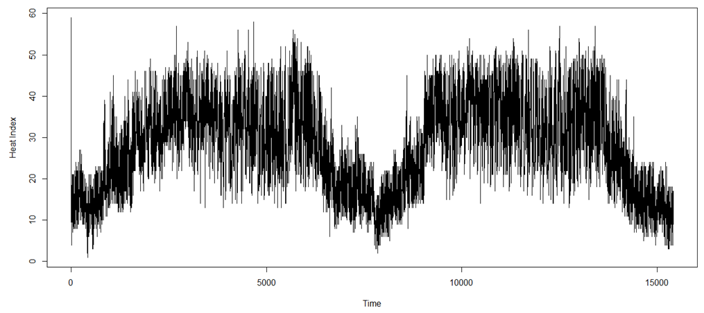
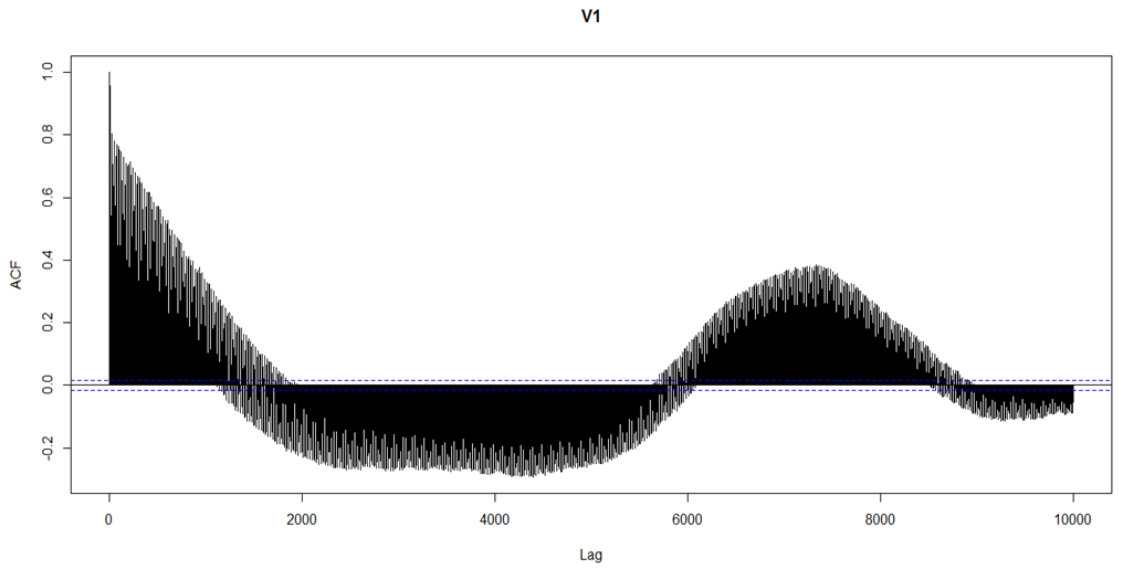
Figure 3.1 reveals the embedded long range dependency characteristics of the hourly data points in KEBBI between 2013/14. The data are highly correlated, there is a sense of return of a particular characteristic after some hours and this depicts seasonality traits and fractional integrated d series suspected. There was a drop after the first seven thousand hours of which it now picks and falls after fifteen hours, also the graph point shows the tendency of high correlation between the set of data point which amount to the fact the series is stable over time.

Figure 3.1. Visual Representation of Hourly Heat Index in KEBBI between 2013 and 2014

Figure 3.2. Visual Representation of First Two Thousand Five Hundred Hours Observation

The autocorrelation function of the first two thousand five hundred (2500) observations in the data set displayed a trait of seasonality as it can be seen in the figure above that for every lag multiple of twelve (600) there appeared trough and picks, very strong correlation was noticed.

The figure 3.3 revealed that when the number of the lag is double we have a longer turning point, very strong correlation was noticed.

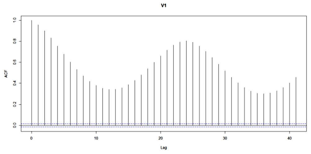
Figure 3.3. Visual Representation of Five Thousand Hours Observations

The figure 3.4 shows that there is a very strong correlation among the data points and the sinusoidal movement imitates a seasonal trait.

Figure 3.4. Visual Representation of Ten Thousand Hours Observations

Table 3.1. Descriptive Statistics for the Heat Index at Different Hours

Table 3.1 shows the descriptive statistics of the heat index where the all samples are sub divided in three categories the first two thousand five hundred observations, five thousand observations and ten thousand observations; in order to examine the characteristics of the integrated order of at different sample hours. The minimum value of heat index for the hall sample is 1 and the maximum is 59. The average mean of the hall sample is 27.72.

Table 3.2. Portmanteau Test for Autocorrelation

The table 3.2 above shows the results of the Portmanteau test at lag interval of 200 of which the first 21 of them are displayed. It reveals highly correlated set of data points which connotes non stationary level of the series.

Table 3.3. ADF Test for the Long Memory Process

The result from dickey fuller appears as if the series of apparent temperature is stationary unfortunately however, it is a long memory process where the value of the integrated order d in this case is not unit rather, a fractional value.

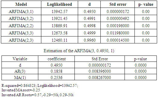
Having searched the ARFIMA models in an interval of [0,3] for both orders of p and q with fractional integrated using Schwarz Information Criterion, the ARFIMA(3, 0.4950, 1) tend to be the most preferable model, the results are displayed in Table 3.4 below.

Table 3.4. Selection of ARFIMA Models

4. Discussion of Results

The research investigated the long range dependency characteristics of apparent temperature in Birnin Kebbi using ARFIMA model. The plots and the original autocorrelation structure are carefully examined and it is evident from the ADF test that the series under investigation does not contain unit root, neither can it be associated with a stationary to a series. It is noticed from the preliminary investigation the series possess long range dependency characteristics of d lying between 0 and 0.5 using Geweke, et al (2008) estimator and ARFIMA. ARFIMA model gives a better estimate. Long range dependency tend to reflect the persistence of shock in a very long time period after it occurs, meaning that; once a shocks is felt on the apparent temperature, it will go onto a very long time period for which the pattern or structure will be repeated. This can also be seen in the autocorrelation structure of all samples and when it is sub divided in to three categories, the average time of return is three hundred and twelve days which is approximately one year to all samples. Sample 2500 showed asinusoidal pattern in the structure, while samples 2500, 5000 and 10000 imitated the repetitive nature of shock persistence after a very long period of time. This shows that there is always a period where the apparent temperature is at pick or at lowest point. This research work prevent the misleading integrated of d = 1 for ARIMA process.

5. Conclusions

The research was set out to investigate the long memory behaviour of apparent temperature in KEBBI metropolis, KEBBI State using hourly data for a period of two years (2013/14). Time series methodology of Autoregressive Fractional Integrated Moving Average model (ARFIMA) is used in the study. The results revealed that the series for the period investigated is highly correlated and fractionally integrated with the value of d is 0.495 and the number of days for the return characteristics of the persistence of the shock is estimated to be 312 days approximately a year.