1. Introduction

Let a random variable has probability distribution . If sample units are weighted or selected with probability proportional to , then the corresponding size-biased distribution of order is given by its probability mass function (pmf)

(1.1)

where . When , the distribution is known as simple size-biased distribution and is applicable for size-biased sampling and for , the distribution is known as area-biased distribution and is applicable for area-biased sampling. In many statistical sampling situations care must be taken so that one does not inadvertently sample from size-biased distribution in place of the one intended.

Size-biased distributions are a particular case of weighted distributions which arise naturally in practice when observations from a sample are recorded with probability proportional to some measure of unit size. In field applications, size-biased distributions can arise either because individuals are sampled with unequal probability by design or because of unequal detection probability. Size-biased distributions come into play when organisms occur in groups, and group size influences the probability of detection. Fisher (1934) firstly introduced these distributions to model ascertainment biases which were later formalized by Rao (1965) in a unifying theory for problems where the observations fall in non-experimental, non-replicated and non-random categories. Size-biased distributions have applications in environmental science, econometrics, social science, biomedical science, human demography, ecology, geology, forestry etc. Further, size-biasing occurs in many unexpected context such as statistical estimation, renewal theory, infinite divisibility of distributions and number theory. Van Duesen (1986) has detailed study about the applications of size-biased distributions for fitting distributions of diameter at breast height (DBH) data arising from horizontal point sampling (HPS). Later, Lappi and Bailey (1987) have applied size-biased distributions to analyze HPS diameter increment data. The applications of size-biased distributions to the analysis of data relating to human population and ecology can be found in Patil and Rao (1977, 1978). A number of research have been done relating to size-biased distributions and their applications in different fields of knowledge by different researchers including Scheaffer (1972), Patil and Ord (1976), Singh and Maddala (1976), Patil (1981), McDonald (1984), Gove (2000, 2003), Correa and Wolfson (2007), Drummer and McDonald (1987), Ducey (2009), Alavi and Chinipardaz (2009), Ducey and Gove (2015), are some among others.

Shanker (2015) introduced one parameter Akash distribution having probability density function (pdf) and cumulative distribution function (cdf)

(1.2)

(1.3)

for modeling various lifetime data from biomedical science and engineering. Shanker (2015) has discussed its various interesting and important properties, estimation of parameter and applications.

Assuming the parameter of the Poisson distribution to follow Akash distribution (1.2), Shanker (2017) introduced Poisson-Akash distribution (PAD), a Poisson mixture of Akash distribution, having pmf

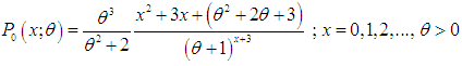(1.4)

Various statistical properties of PAD, estimation of parameter and applications to model count data have been studied by Shanker (2017) and it has been observed that it gives better fit than both Poisson distribution and Poisson-Lindley distribution, a Poisson mixture of Lindley (1958) distribution and introduced by Sankaran (1970). The first four moments about origin and the variance of PAD obtained by Shanker (2017) are given by

2. Size-Biased Poisson-Akash Distribution

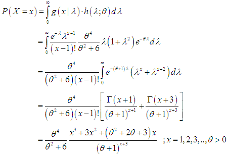
Using (1.1) and (1.4) and the expression for the mean of PAD, the size-biased Poisson-Akash distribution (SBPAD) with parameter can be defined by its pmf

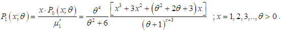(2.1)

Recall that the pmf of SBPAD (2.1) can also be obtained from the size-biased Poisson distribution (SPBD) with pmf

(2.2)

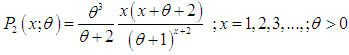
when its parameter follows size-biased Akash distribution (SBAD) with pdf

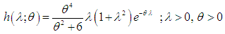(2.3)

Thus the pmf of SBPAD can be obtained as

(2.4)

which is the pmf of SBPAD obtained in (2.1).

It can be easily verified that SBPAD is unimodal and have increasing failure rate. Since

is a deceasing function of is log-concave. Therefore, SBPAD is unimodal, has an increasing failure rate (IFR), and hence increasing failure rate average (IFRA). It is new better than used in expectation (NBUE) and has decreasing mean residual life (DMRL). The definitions, concepts and interrelationship between these aging concepts have been discussed in Barlow and Proschan (1981).

The graphs of the pmf of SBPAD (2.1) for varying values of the parameter have been drawn in figure 1. The graphs have been shown for both starting from and to see the difference in the nature. The graphs starting from are positively biased whereas graphs starting from are monotonically decreasing except for .

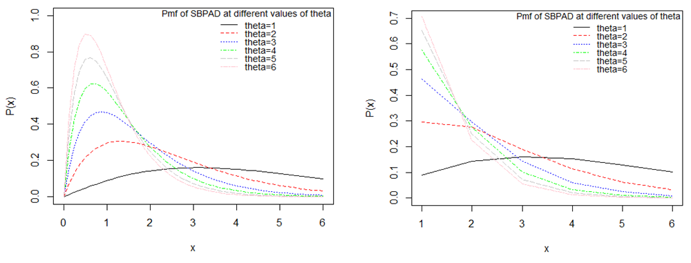Figure 1. Graphs of pmf of SBPAD for varying values of the parameter θ

It would be recalled that the pmf of size-biased Poisson-Lindley distribution (SBPLD) given by

(2.5)

has been introduced by Ghitany and Mutairi (2008), which is a size-biased version of Poisson-Lindley distribution (PLD) introduced by Sankaran (1970). Ghitany and Mutairi (2008) have discussed its various mathematical and statistical properties, estimation of the parameter using maximum likelihood estimation and the method of moments, and goodness of fit. Shanker et al (2015) has critical study on the applications of SBPLD for modeling data on thunderstorms and found that SBPLD is a better model for thunderstorms than size-biased Poisson distribution (SBPD).

3. Moments

Using (2.4), the rth factorial moment about origin of the SBPAD (2.1) can be obtained as

Taking , we get

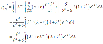Using gamma integral and a little algebraic simplification, the rth factorial moment about origin of SBPAD (2.1) can be obtained as

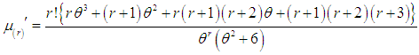(3.1)

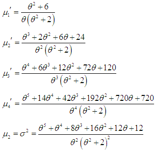
Taking 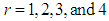in (3.1), the first four factorial moments about origin can be obtained and using the relationship between moments about origin and factorial moments about origin, the first four moments about origin of the SBPAD (2.1) are thus obtained as

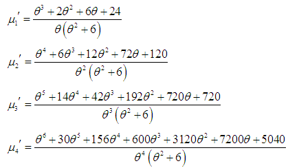Now, using the relationship between moments about mean and the moments about origin, the moments about mean of the SBPAD (2.1) can be obtained as

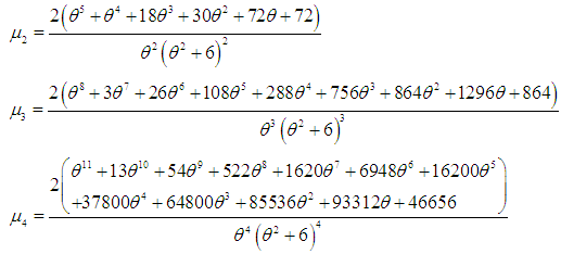The coefficient of variation , coefficient of Skewness , coefficient of Kurtosis and index of dispersion of the SBPAD (2.1) are thus obtained as

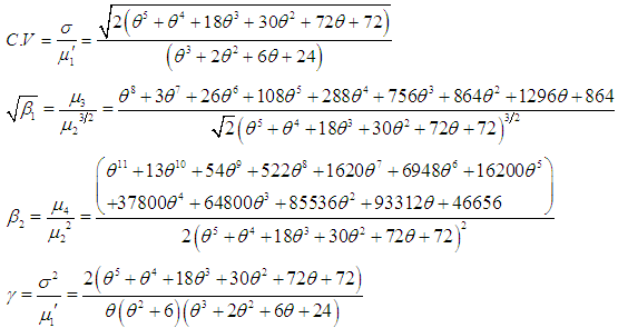The graphs of coefficient of variation , coefficient of Skewness , coefficient of Kurtosis and index of dispersion of the SBPAD are shown in figure 2. From fig. 2, it is obvious that C.V and index of dispersion are monotonically decreasing whereas coefficient of skewness and coefficient of kurtosis are monotonically increasing for increasing values of the parameter .

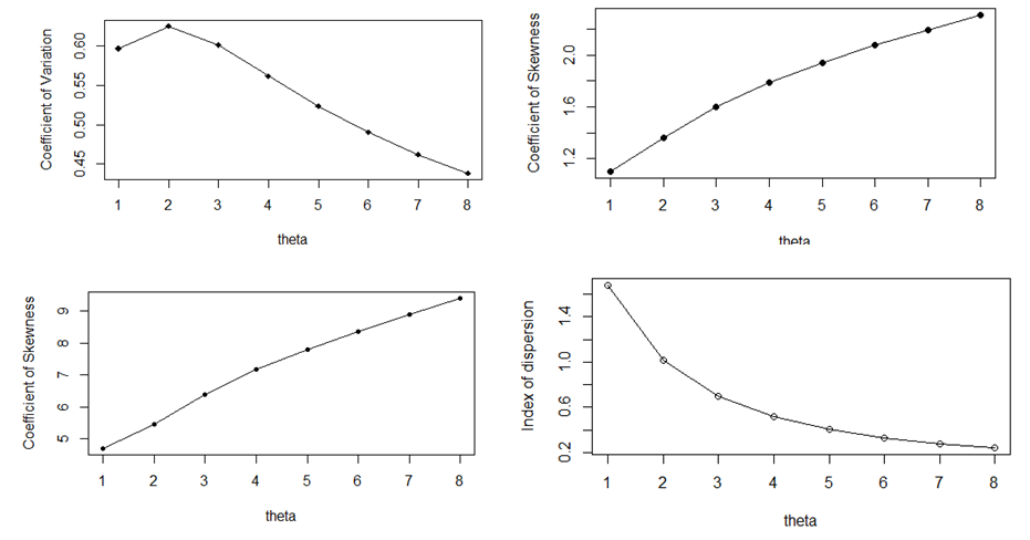Figure 2. Graphs of C.V, coefficient of Skewness, coefficient of Kurtosis and index of dispersion of the SBPAD for varying values of the parameter θ

It can be easily verified that SBPAD is over-dispersed , equi-dispersed and under-dispersed for 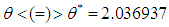. It should be noted that SBPLD is over-dispersed , equi-dispersed and under-dispersed for .

4. Estimation of Parameter

4.1. Method of Moment Estimate (MOME): Equating the population mean to the corresponding sample mean, the method of moment estimate (MOME) of of SBPAD (2.1) is the solution of the following cubic equation in

, where is the sample mean.

4.2. Maximum Likelihood Estimate (MLE): Let be a random sample of size n from the SBPAD (2.1) and let be the observed frequency in the sample corresponding to such that , where is the largest observed value having non-zero frequency. The likelihood function of the SBPAD (2.1) is given by

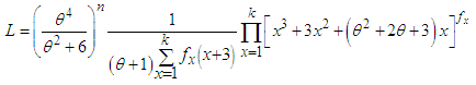The log likelihood function can be obtained as

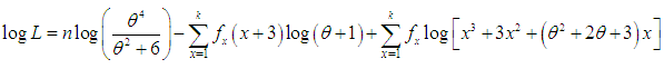The first derivative of the log likelihood function is thus given by

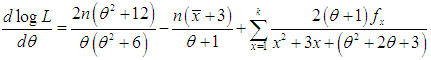where is the sample mean.

The maximum likelihood estimate (MLE), of of SBPAD (2.1) is the solution of the equation and is given by the solution of the following non-linear equation

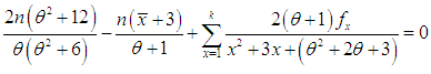This non-linear equation can be solved by any numerical iteration methods such as Newton- Raphson method, Bisection method, Regula –Falsi method etc. In the present paper, Newton-Raphson method has been used to solve the above non-linear equation to find MLE of the parameter. Note that the MLE of the parameter θ is the local solution and it does not matter much because accuracy of the estimate has been considered.

5. Goodness of Fit

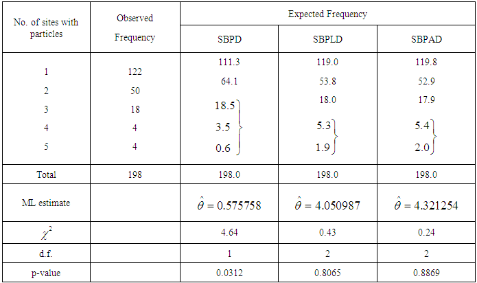
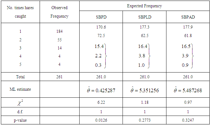
In this section the goodness of fit of SBPAD, SBPLD and SBPD has been presented for two count datasets. The fit of these distributions are based on maximum likelihood estimates of the parameter. The first dataset is immunogold assay data of Cullen et al. (1990) regarding the distribution of number of counts of sites with particles from immunogold assay data, the second dataset is animal abundance data of Keith and Meslow (1968) regarding the distribution of snowshoe hares captured over 7 days.

The fitted plots of the SBPD, SBPLD and SBPAD for datasets in table 1 and 2 are shown in figure 3. From the fitted plot of the distributions, it is also obvious that SBPAD is closer to the observed values than SBPD and SBPLD and hence SBPAD has advantage over these distributions for modeling count data excluding zero counts.

Table 1. Distribution of number of counts of sites with particles from Immunogold data

Table 2. Distribution of snowshoe hares captured over 7 days

Figure 3. Fitted plots of the SBPD, SBPLD and SBPAD for datasets in table 1 and 2

6. Concluding Remarks

In the present paper size-biased Poisson-Akash distribution (SBPAD), a simple size-biased version of the Poisson-Akash distribution (PAD) of Shanker (2017), has been proposed and studied. Its raw moments and central moments have been obtained and hence expressions for coefficient of variation (C.V.), skewness, kurtosis and index of dispersion have been presented and their natures have been discussed graphically. The estimation of its parameter has been discussed using the method of moments and the method of maximum likelihood estimation. The goodness of fit of the SBPAD has been discussed with two examples of observed real datasets over SBPD and SBPLD and the fit given by SBPAD gives quite satisfactory fit. Therefore, SBPAD can be considered an important distribution for modeling count data excluding zero counts over SBPD and SBPLD.

ACKNOWLEDGEMENTS

The author is grateful to the Editor-In-Chief of the journal and the anonymous reviewer for their constructive suggestions which improved the presentation and the quality of the paper.