-
Paper Information
- Previous Paper
- Paper Submission
-
Journal Information
- About This Journal
- Editorial Board
- Current Issue
- Archive
- Author Guidelines
- Contact Us
International Journal of Statistics and Applications
p-ISSN: 2168-5193 e-ISSN: 2168-5215
2017; 7(6): 280-288
doi:10.5923/j.statistics.20170706.02

Modeling Sugarcane Yields in the Kenya Sugar Industry: A SARIMA Model Forecasting Approach
 Abstract
 Reference
 Full-Text PDF
 Full-text HTML
Mwanga D.1, Ong’ala J.2, Orwa G.1
1Department of Statistics and Actuarial Science, Jomo Kenyatta University of Agriculture and Technology, Juja, Kenya
2Department of Mathematics, Masinde Muliro University of Science and Technology, Kenya
Correspondence to: Mwanga D., Department of Statistics and Actuarial Science, Jomo Kenyatta University of Agriculture and Technology, Juja, Kenya.
| Email: |  |
Copyright © 2017 Scientific & Academic Publishing. All Rights Reserved.
This work is licensed under the Creative Commons Attribution International License (CC BY).
http://creativecommons.org/licenses/by/4.0/

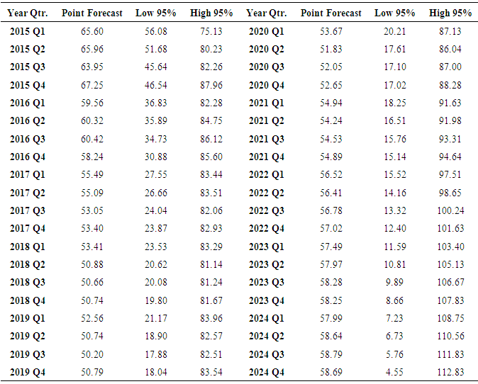
The purpose of this study was to fit a model that forecasts quarterly sugarcane yields in Kenya. Seasonal ARIMA models are explored and tested. Seasonal ARIMA(2,1,2)(2,0,3)4 is found to be the best model that fits quarterly sugarcane yields from 1973-2015. Sugarcane yields data collected quarterly from 1973-2014 is used for modeling and SARIMA (2,1,2)(2,0,3)4 model is fit and 2015 quarterly forecasts are compared against the actual quarterly yields in 2015. If all factors are held constant, the model predicted a drop in sugarcane yields in 2016 to 60 (95% CI: 34.58, 84.69) tonnes of cane per hectare (tch) in 2016, 54 (95% CI: 26.24, 82.43) tch in 2017 and 51.48 (95% CI: 21.51, 81.45) tch in 2018. A steady increase would be observed again from 2020-2024.
Keywords: Seasonal ARIMA, Exponential smoothing, Forecast, Sugarcane yields
Cite this paper: Mwanga D., Ong’ala J., Orwa G., Modeling Sugarcane Yields in the Kenya Sugar Industry: A SARIMA Model Forecasting Approach, International Journal of Statistics and Applications, Vol. 7 No. 6, 2017, pp. 280-288. doi: 10.5923/j.statistics.20170706.02.
Article Outline
1. Introduction
- Historical BackgroundSugarcane is an important commercial crop grown in four major sugarcane growing belts in the Kenya such us; Central Nyanza, Western Kenya, South Nyanza and the Coast. Before independence, the sugar industry in Kenya was dominated by the private sector. Historically, the growing of sugarcane in Kenya started with the involvement of the Kenya Government at the turn of the century, with the establishment of experimental farms at Mazeras and Kibos, whose sole activity was to evaluate sugarcane and other introduced crops. Subsequently, large production of sugarcane started in 1923 when a sugar factory was built at Miwani in Nyanza Province, Kisumu District and at Ramisi in Coast Province, Kwale District. Today sugarcane is grown for white sugar production in Nyando, South Nyanza, Mumias, Nzoia and Busia by small, large scale farmers and sugar factories. Sugarcane yields have declined in the past decade with average tones cane per hectare (tch) dropping from 74 tch in 2004 to 61 tch in 2014 [1]. The total area under cane was approximately 211,342 hectares in 2014 compared to 213,920 hectares in 2013 [2]. This decline has had adverse effects directly on the livelihood of sugarcane farmers who directly depend on sugarcane farming. Sugarcane farmers have experienced many challenges over time and many have since threatened to pull out of sugarcane farming and explore other profitable farming practices [3]. There are many studies that have been done in order to help secure the industry from falling which includes studies that have been conducted by Kenya Agricultural and Livestock Research Organization-Sugar Research Institute (KALRO-SRI), the institution mandated to carry out research in sugar and sugarcane. They range from studies on best management practices, drainage and irrigation, farmers’ trainings, trainings of trainers (ToTs), coping strategies to the challenges facing the industry, studying and releasing new and improved varieties, development of a synchrony model to help the millers bridge the gap between factory crushing capacity and harvesting time and many others. However, the adoption of these technologies by the farmers and the sugarcane millers has however not been very encouraging [4] [5]. This is generally contributed by the low motivation farmers have developed towards sugarcane farming more often associating it with poverty and feeling that sugarcane farming is not productive.Forecasting Methods in the Kenya Sugar IndustryThere are limited studies in Kenya that have explored the forecasting methods on sugarcane production in the Kenya with the view to improve or develop new methods. This necessitates the need to develop models and methodologies that would be useful to predict sugarcane yields and its components.Since sugarcane was first grown in Kenya, sugarcane yield is estimated using conventional approaches through biennial field surveys by the millers and the sugar directorate. Their methodology is based on visual physical assessment [2, 6]. In this method, a monthly productivity index ranging between 0 to 5 is applied to sample cane crop from the age of one month while considering the parameters; crop vigour, crop colour, crop density, weed status, pests and diseases at the time of the assessment. The estimated yield is then used to project sugarcane production for the current and the subsequent year. Mulianga et al. (2013) explored the suitability of the Normalized Difference Vegetation Index (NDVI) from the Moderate Resolution Imaging Spectrometer (MODIS) obtained for six sugar management zones, over nine years (2002–2010), to forecast sugarcane yield on an annual and zonal base. They took into account the characteristics of the sugarcane crop management (15-month cycle for a ratoon, accompanied with continuous harvest in Western Kenya), the temporal series of NDVI was normalized through an original weighting method that considered the growth period of the sugarcane crop (wNDVI), and correlated it with historical yield datasets. They found out that results when using wNDVI were consistent with historical yield and significant, while results when using traditional annual NDVI integrated over the calendar year were not significant [7].Time Series modelingA time series is a sequence of data points, typically consisting of successive measurements made over a time interval. Time series analysis accounts for the fact that data points taken over time may have an internal structure (such as autocorrelation, trend or seasonal variation) that should be accounted for. Sugarcane yields when taken at equal time intervals over a period of time constitute a time series data which could then be analyzed using time series techniques. Presently, statistical techniques of time series analysis have been widely discussed in the literature and there is a great variety of circumstances of research in which they can be used, especially in studies involving time dependent data. Time series models were first introduced by Box and Jenkins in 1960 hence the name Box-Jenkins Model [8]. Originally, Box and Jenkins methodology involved three iterative steps viz; model selection, parameter estimation, and model checking [8-10]. Recent development to this was to add a preliminary stage of data preparation and a final stage of model application which is forecasting [11]. Data preparation in this sense involves transformations and differencing if the data under study require that it be done to satisfy the Box and Jenkins assumptions before modeling. Model selection involves using graphs and model selection tools such as Akaike Information Criteria and Bayesian Information Criteria to identify the model that best fits the data. Parameter estimation means finding the values of the model coefficients which provides the best fit to the data. Model checking means testing for assumptions to identify areas of model inadequacy which in this case involves testing whether residuals are white noise. Once the model has been selected, estimated and checked, it is then used for forecasting [12].A time series
 is a function of any or all of the four components; trend
  , seasonal
  , cyclic
  and a random term
  [13]. This is represented in equation 1.
 | (1) |
 can be multiplicative (equation 2) or additive (equation 3) depending on the series under study.Multiplicative
 | (2) |
 | (3) |
 | (4) |
 | (5) |
 is the time series observation at time t,
  is white noise, μ is the mean of the series,
  is seasonal AR parameters,
  is non-seasonal AR parameters,
  is the seasonal MA parameters,
  is non-seasonal MA parameters, and B is the back shift operator.The back shift operator B can be simplified in AR and MA terms as;
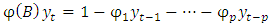 | (6) |
 | (7) |
 | (8) |
 | (9) |
 | (10) |
 | (11) |
2. Materials and Methods
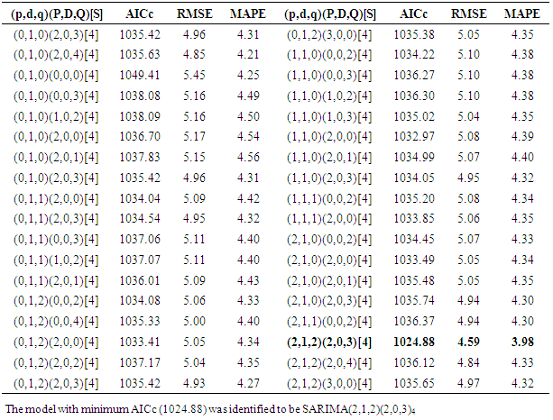
- The data used in this study are secondary data on sugarcane yields collected from Agriculture, Food and Fisheries Authority - Sugar Directorate (AFFA-SD) Year books of Statistics. Sugar Directorate collects and analyzes data on sugar and sugarcane from all the sugarcane growing zones and mills in the Kenya sugar Industry annually. The data is then published in the yearbooks of statistics and shared with agriculture research institutions and other stakeholders for consumption. This study focuses on quarterly sugarcane yield in terms of tones cane per hectare (tch) collected from the Sugar Directorate yearbooks of statistics from 1973-2015. The data were available annually from 1973-2015 and quarterly from 1999-2015. Quarterly data from 1973-1998 were obtained through interpolation using the “zoo” package [22] available in the R software using the available annual data. The “zoo” package has the ability to interpolate missing data without interfering with the underlying trends in the time series. The time series is explored to identify any underlying patterns or behaviors. This is done by decomposing the time series to extract the trend, seasonality and the cyclic components using classical and Seasonal and Trend decomposition using Loess (STL) [23] approaches.Box-Jenkins SARIMA models are explored following all the stages required in Box and Jenkins modeling technique and the best predictive model chosen that will forecast the quarterly sugarcane yields in the Kenya Sugar Industry. Model selection is based on the bias corrected Akaike Information Criteria (AICc) [24] where the model with minimum AICc is selected. Data from 1973 – 2014 is used to fit the SARIMA model and data from the four quarters of 2015 are used to check the adequacy of the forecast. Model diagnostic checking is done by analyzing the residuals. Ljung-Box test for independence of the residuals is done where residuals should be uncorrelated and look like white noise [25].
3. Results and Discussion
- Quarterly sugarcane yields data from 1973-2014 had an average of 76.68 tch (SD=16.51). There was larger variation in the earlier years (1973-2000) with an average of 82.19 tch (SD=17.02) compared to 65.64 tch (SD=7.52) from 2001-2014. Figure 1 shows the plot of the time series.
 | Figure 1. Plot of quarterly sugarcane yields |
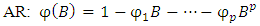
 | Figure 2. Decomposition of time series using STL |
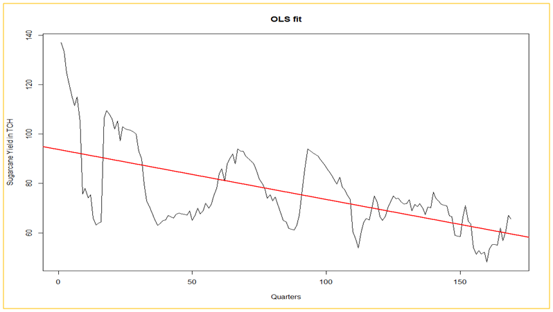 | Figure 3. Trend plot of sugarcane yields from 1973-2015 |
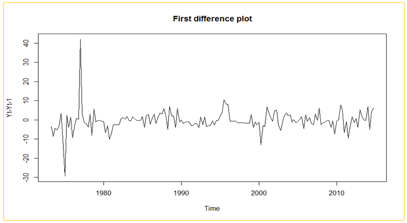 | Figure 4. Plot of the first difference for the time series |
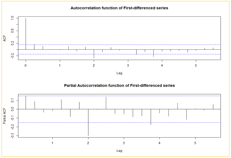 | Figure 5. Estimated ACF and PACF for the differenced time series |
|
|
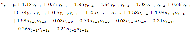 | (12) |
 the estimate of sugarcane yield at time t,
  is the mean time series process,
  is the past observations and
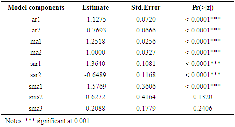
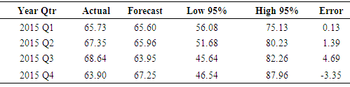
  are the random shocks.Model diagnostic checkingThe third stage in Box and Jenkins modeling is model diagnostic checking that requires that the residuals look like white noise and uncorrelated. The Ljung Box test for autocorrelation indicate independence of the residuals (χ2= 0.5430, df = 1, p-value = 0.4612). Shapiro Wilk’s test for normality also showed that the residuals were approximately normal (W = 0.9891, p-value = 0.2234).ForecastingIn this study SARIMA(2,1,2)(2,0,3)4 was identified as the best fit and thus used for forecasting. Forecasts and actual values for the all the quarters of the year 2015 together with their 95% confidence intervals are given in the in table 3.
|
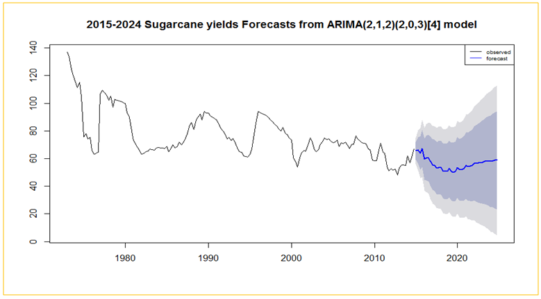 | Figure 6. A 10- year forecast from SARIMA(2,1,2)(2,0,3)4 |
|
4. Conclusions
- The main objective of this study was to identify a model that fits quarterly sugarcane yields data and forecast future yields based on the past values. This study found SARIMA(2,1,2)(2,0,3)4 as the best model which had the lowest AICc and therefore fit to the quarterly sugarcane yields data from 1973-2014. The four quarters of the year 2015 were used to check the adequacy of the model. If all factors remain constant the model predicted a fall in yields until the year 2020 before starting to steadily rising again. Seasonal ARIMA models are proving to be good candidates of modeling time series with seasonal patterns and can be applied in any sector.
ACKNOWLEDGEMENTS
- I acknowledge the Sugar Directorate and for making available the sugarcane yields data available in their annual yearbooks of Statistics and the Sugar Research Institute where from the individual Yearbooks of Statistics were accessed.