M. T. Nwakuya, M. A. Ijomah
University of Port Harcourt, Rivers State, Nigeria
Correspondence to: M. T. Nwakuya, University of Port Harcourt, Rivers State, Nigeria.
| Email: |  |
Copyright © 2017 Scientific & Academic Publishing. All Rights Reserved.
This work is licensed under the Creative Commons Attribution International License (CC BY).
http://creativecommons.org/licenses/by/4.0/

Abstract
Panel data analysis enables the control of individual heterogeneity to avoid bias in the resulting estimates. Using the R software, the fixed effects and random effects modeling approach were applied to an economic data, “Africa” in Amelia package of R, to determine the appropriate model. Taking into consideration the assumptions of the two models, both models were fitted to the data. The Lagrange Multiplier test (Breusch-Pagan) carried out on the estimates of the random model showed that the random model was appropriate for the data, but the model had a low coefficient of determination, R2 of 0.48697. The fixed effect was then estimated using four different approaches (Pooled, LSDV, Within-Group and First differencing) and testing each against the random effect model using Hausman test, our results revealed that the random effect were inconsistent in all the tests, showing that the fixed effect was more appropriate for the data. Among the fixed effects models, the LSDV showed to be the best fit with an R2 of 0.8851.
Keywords:
Fixed effects, Random effects, Coefficient of determination, Panel data and Hausman test
Cite this paper: M. T. Nwakuya, M. A. Ijomah, Fixed Effect Versus Random Effects Modeling in a Panel Data Analysis; A Consideration of Economic and Political Indicators in Six African Countries, International Journal of Statistics and Applications, Vol. 7 No. 6, 2017, pp. 275-279. doi: 10.5923/j.statistics.20170706.01.
1. Introduction
Panel data consists of a group of cross-sectional units who are observer over time, [8]. It is a marriage of time series and cross sectional data, in other words there will be space as well as time dimensions. Some literatures refer to it as pooled data (pooling of cross section and times observations), longitudinal data (the study of a group of variables over time), event history analysis (studying the movement over time of subjects through successive states or conditions), cohort analysis (studying a particular sect over time) etc. Examples of panel data include; annual unemployment rates of each state over several years, quarterly sales of individual stores over several quarters etc. Panel data are more informative (more variability, less collinearity, more degrees of freedom), estimates are more efficient it minimizes bias due to aggregation, [3]. It allows the study of individual dynamics (e.g separating age and cohort effects). It also allows the control for individual unobserved heterogeneity; however it increases the complexity of the analysis. Panel data can be balanced or unbalanced, short or long panel. A balanced panel data is one in which each subject (firm, individuals etc) has the same number of observations. If each subject has a different number of observations, then we have an unbalanced data. In short panel the number of cross-section subjects, N, is greater than the time periods T. While in a long panel the time period is greater than the number of cross-sections [7].Majorly panel data is analyzed using either fixed effect or random effect [8]. Researchers are always in the dilemma of deciding which one to use. While debates continue within about which approach is best for certain situations, [1], [2], [19].In this paper we tried to highlight the application of both fixed effect and random effect in a particular data set and also various tests to determine the more suitable one for the data set presented in this work.
2. The Models
Panel data it makes conceptual contrasting assumptions about effects as either random or fixed, [4]. Our model is given by;  | (1.1) |
Where X stands for the four Economic and Political Indicators in six African Countries, namely; Inflation, trade, civil liability and population. i stands for ith Country, i=1,..6 (Burkina faso, Burundi, Cameroon, Congo, Senegal and Zambia.), t stands for tth time period, i=1,..,T (1972-1991).
2.1. Pooled OLS Regression Model
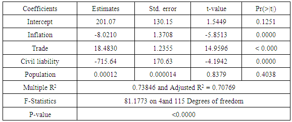
In pooled OLS regression, we simply pool all observations and estimate the grand regression, ignoring the cross-section and time series nature of the data, in which case the error term captures everything. In this model because observations were pooled together it camouflages the heterogeneity or individuality that exists between the variables, [8].Table 1.1. Pooled Regression model estimates
 |
| |
|
2.2. The Fixed Effect Model
The fixed-effects model controls for all time-invariant differences between the individuals, so the estimated coefficients of the fixed-effects models cannot be biased because of omitted time-invariant characteristics…[like culture, religion, gender, race, etc]. Stock and Watson [17], gave an insight that if the unobserved variable does not change over time then any changes in the dependent variable must be due to influences other than the fixed characteristics. One of the concerns practitioners raise about the fixed effect model is that it eats up too many degrees of freedom, resulting in shaky estimates, [1]. This is somewhat of a misconception. Another side effect of the features of fixed-effects models is that they cannot be used to investigate time-invariant causes of the dependent variables. That is, one cannot retrieve “good” estimates of sluggish, or slowly-changing, variables in the fixed effect model. Technically, time-invariant characteristics of the individuals are perfectly collinear with the person [or entity] dummies. Substantively, fixed-effects models are designed to study the causes of changes within a person [or entity]. A time-invariant characteristic cannot cause such a change, because it is constant for each person.” An important assumption of the fixed effect is that, those time invariant characteristics is unique to the individual and should not be correlated with other individual characteristics. Each entity is different therefore the entity’s error term and the constant (which captures individual characteristics) should not be correlated with the others. If the error terms are correlated the fixed effect is not suitable.
2.3. The Fixed Effect Least-Square Dummy Variable Model (LSDV)
Given eqn1.1, each country i has T observations and there are i=1,…,6 countries. Several kinds of fixed effects differ in the assumptions about, the intercept and the slope coefficients. Introducing dummy variable is the simplest method of isolating individual or time specific effect in a regression model. The individual effect is picked up by the dummy variable Dmi where m = n-1.Ÿ Fixed effect model with dummy variables, where intercepts are different for different countries  , but each individual intercept does not vary over time.
  | (1.2) |
Since the number of countries are N = 6 we have; | (1.3) |
Where the dummy variables are defined thus;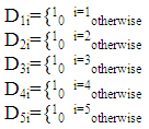
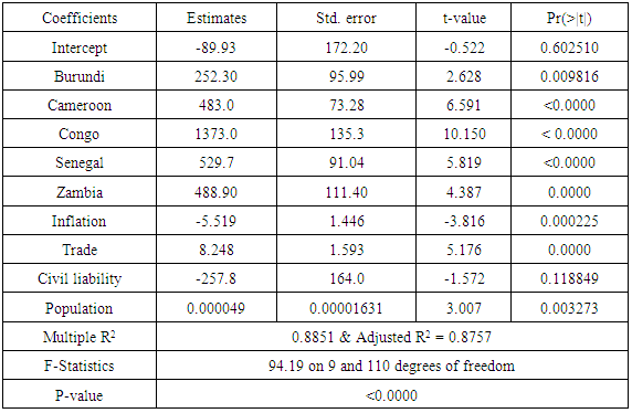
Table 1.2. LSDV model Estimates
 |
| |
|
Ÿ Fixed effect model with dummy variables, where intercepts are different for different time periods  , Since the number of countries T = 20 we have;
 | (1.4) |
The number of interaction terms is number dummy variables and number of explanatory variablesŸ Fixed effect model with dummy variables, where both intercept and slope vary over individuals and time, this requires a lot of variables.
2.4. Fixed Effects Within-Group Model
The technique of including a dummy variable for each variable is feasible when the number of individual N is small. However if the number of individual is large this will not work, because there will be too many dummy variables. To estimate fixed effect with large sample size we have, for the regression model below;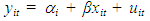 | (1.5) |
Averaging over time gives; | (1.6) |
Where 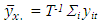 and
and  Therefore subtracting equation (1.8) from (1.7) gives;
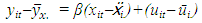 | (1.7) |
This gives rise to the transformed model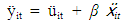 | (1.8) |
Where; 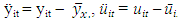 and
and  Fixed effect within group estimator for β is;
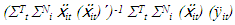 | (1.9) |
We can see in eqn (1.7) that by subtracting the means we have restricted all of the action in the regression within-group. Thus we have eliminated the key source of omitted variable bias that is the unobservable across-group differences [11]. Table 1.3. Within-Group Model Estimates
 |
| |
|
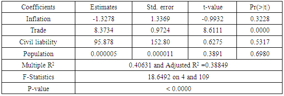
2.5. The Fixed Effect First Difference Model
The first difference estimator wipes out time invariant omitted variables using the repeated observations over time, [4].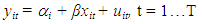 | (2.0) |
 | (2.1) |
Differencing both equations, gives the model | (2.2) |
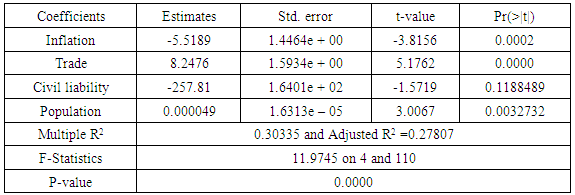
The First Difference estimator β= (∆X´∆X)-1∆X´∆yTable 1.4. First Difference Model Estimates
 |
| |
|
2.6. Random Effects Model
The rationale behind random effects model is that the individual-specific effect or variation across entities is assumed to be a random variable that is uncorrelated with the predictor/explanatory variables: “…the crucial distinction between fixed effect and random effect is whether the unobserved individual effect embodies elements that are correlated with the regressors in the model, not whether these effects are stochastic or not” [6]. An advantage of random effects is that you can include time invariant variables like gender, unlike in fixed effect, where the intercept absorbs all the time invariant variables. Here the individual’s error term is not correlated with the predictors which allows for time invariant variables to play a role as explanatory variables. By specifying the intercept parameters αi (in equation 1.7) to consist of a fixed part that represents the population average  and a random individual difference from the population average, eit, this is broken down as:
  . The random individual differences eit called the random effects, are analogous to random error terms, and it is assumed that they have zero mean, are uncorrelated across individuals and they also are assumed to have constant variance, σ2e, so that; E(ei) = 0, cov(ei ej) = 0 and var(ei)= σ2e if this is substituted in equation 1.7, we will have;
  | (2.3) |
Rearranging we have; | (2.4) |
where, vit is the combined error term (eit+uit), because of this combined error term, this model is often referred to as error component model. The random effects allow the generalization of the inferences beyond the sample used in the model. The random effects model is a “partial pooling” approach, with the effects of X1ij and X2ij being a weighted average of the within and between-cluster variation in the data [5], [8], [9], [15]. The random effects approach, and the more generalized random coefficient model, is widely used in analyses of panel data (with large N relative to T) and multilevel data [12], [16]. A major complaint lodged against the random effects model relates to the restrictive assumption that level-1 independent variables be uncorrelated with the random effects term: Cov(Xij, u0j) = 0. Since a level-1 variable varies both within and between clusters, many argue that this an unrealistic assumption to satisfy, since unobserved heterogeneity will almost always be correlated with the independent variables. This controversial assumption often makes the fixed effect model, which does not incorporate this assumption, a superior choice over the random effects model [1], [10], [19].
3. Tests
3.1. Random Effects Test
Hill [8], showed that the two errors are correlated over time for a given individual but are otherwise uncorrelated. They went further to say that the correlation is caused by the component of ei that is common to all time periods and it is constant over time and does not decline as the observations get further apart in time. This correlation ρ= σ2e/ (σ2u+ σ2e), it gives the proportion of the variance in the total error term vit that is attributable to the variance of the individual component et. Hill [8] stated that the magnitude of the correlation ρ is a very important aspect of the random effects, if σ2e =0 it means ρ = 0 and there is no random individual heterogeneity present in the data. The presence of individual heterogeneity can be tested by testing the null hypothesis. H0: σ2e Vs H1: σ2e > 0. If the null hypothesis is rejected, then we conclude that there is individual heterogeneity that means that the random effects model is appropriate. The Lagrange Multiplier principle is most convenient and appropriate for testing for individual heterogeneity. The test statistic is due to Breusch and Pagan and is given for balanced as; | (2.5) |
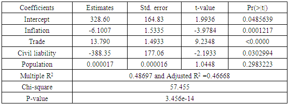
[8], where N is total observations and T is the total time period, LM~χ2(1) if the hypothesis is true. The null hypothesis is rejected and the alternative accepted if LM ≥ χ2(1-α,1) and the conclusion is that there is presence of random effects.Table 1.5. Random Effects Model Estimates
 |
| |
|
3.2. Hausman’s Test
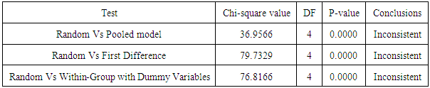
Using the Hausman’s test we compared the random effects model to the fixed effects models, the results are shown in the table (1.6), the table shows that the random effects model was inconsistent when compared to the pooled regression model, LSDV model, First difference and Within-Group fixed effect model. Table 1.6. Hausman’s test
 |
| |
|
4. Results
The least square estimates for the pooled data is given in table (1.1). From the table the country intercepts vary considerably, suggesting that the assumption of differing intercepts for different countries is appropriate. To confirm this fact we ran the following test for the hypothesis below.Ho: β11 = β12 = … β1N H1: Atleast one β1i is differentThe value for F-statistic = 81.1773, yielding a p-value of 2.2e-16; the null hypothesis that the intercepts are equal for all countries was rejected. Based on the differences in the country intercepts, we conclude that the data should not be pooled. The Lagrange Multiplier test (Breusch-Pagan) carried out on the estimates of the random model showed that the random model was appropriate for the data, with a chi-square of 57.455 and a P-value of 3.456e-14, showing that random effects were present, but the estimates of the random effects model shown in table (1.5), with an R2 of 0.48697 tells us that the random model is not a very good fit for the data. We then applied the fixed effects models. Adopting the LSDV model given in equation 1.3, table (1.2) shows the estimates for LSDV model, also Table (1.4) shows the estimates of the first difference model with an R2 of 0.40631and also table (1.3) shows the estimates of within group model with an R2 of 0.30335.
5. Conclusions
The Lagrange Multiplier test (Breusch-Pagan) carried out on the estimates of the random model showed that the random model was appropriate for the data, but the model had a low coefficient of determination, R2 of 0.48697. The fixed effect was then estimated using four different approaches (Pooled, LSDV, Within-Group and First differencing) and testing each against the random effect model using Hausman test, our results revealed that the random effect was inconsistent in all the tests, showing that the fixed effect was more appropriate for the data. Among the fixed effects models, the LSDV showed to be the best fit with an R2 of 0.8851.
References
| [1] | Beck, N. L., and Jonathan N. K. (2001), “Throwing Out the Baby with the Bathwater: A comment on Green, Yoon and Kim,” International Organization, 55:487-95. |
| [2] | Beck, N. L., and Jonathan N. K. (2007), “Random coefficient models for time Series cross-Section data: Monte Carlo experiments,” Political Analysis 15:182-195. |
| [3] | Baltagi, B. H. (2001), “Econometric analysis of panel data,” John Wiley & Sons; 5-20. |
| [4] | Bruce E. H. (2016), “Econometrics,” University of Wisconsin press. |
| [5] | Gelman, A. and Jennifer H. (2007), “Data analysis using regression and multilevel/hierarchical models,” New York: Cambridge University Press. |
| [6] | Greene W. H. (2008), “Econometric Analysis,” Prentice Hall, 100-210. |
| [7] | Gujarati D. N. and Porter D. C., (2009), “Basic Econometrics,” McGraw-Hill Companies Inc. New York, 593-607. |
| [8] | Hill R. C., Griffiths W. E. and Lim G.C. (2007), “Principles of Econometrics,” John Wiley & Sons Inc. New Jersey, 382-404. |
| [9] | Hsiao, C. (2003), “Analysis of panel data,” New York: Cambridge University Press. |
| [10] | Kristensen, I. P. and Wawro G. (2003), “Lagging the dog? The robustness of panel corrected standard errors in the presence of Serial correlation and observation specific effects,” Presented at the Political Methodology Conference. |
| [11] | Kurt S., (2016), “Short guides to microeconometrics, panel data, fixed and random Effects,” Available: https://0x9.me/YRDk8. |
| [12] | Martin, A. D. (2001), “Congressional decision making and the Separation of Powers,” American Political Science Review 95:361-378. |
| [13] | Plumper, T, and Troeger. V. E. (2007), “Efficient estimation of time-invariant and rarely changing variables in finite sample panel analyses with unit fixed effects,” Political Analysis 15:124-139. |
| [14] | Shaun, B., Donovan, T. and Hanneman, R. (2003), “Art for democracy’s sake? Group membership and political engagement in Europe,” Journal of Politics, 65:11- 29. |
| [15] | Skrondal, A. and Rabe-Hesketh, S. (2004), “Generalized latent variable modeling: Multilevel, longitudinal, and structural equation models,” Boca Raton, FL: Chapman & Hall. |
| [16] | Steenbergen, M. R., and Bradford S. Jones. (2002), “Modeling multilevel data structures,” American Journal of Political Science 46:218-37. |
| [17] | Stock J. H. and Watson M. W., (2003), “Introduction to Econometrics,” New York, Prentice hall; 289-290. |
| [18] | Wawro, G. (2003), “Estimating dynamic panel models in political science,” Political Analysis 10:25–48. |
| [19] | Wilson, S. E., and Butler, D.M. (2007), “A lot more to do: The sensitivity of time series cross-section analyses to simple alternative specifications,” Political Analysis 15:101-23. |

 Abstract
 Reference
 Full-Text PDF
 Full-text HTML