M. A. Ali, M. S. Albassam
Department of Statistics, Faculty of Science, King Abdulaziz University, Jeddah, KSA
Correspondence to: M. A. Ali, Department of Statistics, Faculty of Science, King Abdulaziz University, Jeddah, KSA.
| Email: |  |
Copyright © 2017 Scientific & Academic Publishing. All Rights Reserved.
This work is licensed under the Creative Commons Attribution International License (CC BY).
http://creativecommons.org/licenses/by/4.0/

Abstract
In this paper, a pooled test statistic for testing the treatment contrasts has been proposed for which groups of experiments are conducted in two way design model with interactions in heterogeneous environments. The empirical distribution, percentile points and some other distributional properties of the proposed test statistic have been found using Monte Carlo study and the results have been compared with the studies of James and others. From the Monte Carlo simulation study, it has been observed that the distribution of the proposed test statistic was not following χ2 distribution or any other known exact distribution in all cases considered. Empirical pdf, cdf curves, percentile points and some other distributional characteristics as well as numerical illustrations along with real data have also been provided in this paper.
Keywords:
Treatment contrast, Heterogeneous environment, Two way classification with interaction, Chi-square distribution, Monte Carlo study and simulation
Cite this paper: M. A. Ali, M. S. Albassam, Pooled Test Statistic for Treatment Contrast under Heterogeneous Environment and Two Way Interaction Design Model, International Journal of Statistics and Applications, Vol. 7 No. 5, 2017, pp. 258-267. doi: 10.5923/j.statistics.20170705.03.
1. Introduction
Experiments may be conducted with the aid of any suitable experimental designs. Researchers have to repeat their experiments several times across different locations, environments or seasons. The reason may be due to lack of space that would accommodate all the experimental plots or with the underlying condition that the experiments must be carried out at different locations (environment) or different seasons. Whatever may be the reason, the major aim was to do pooled analysis of the data obtained from these multi-environments instead of doing the analysis separately or individually (Albassam and Ali, 2014; Jamjoom and Ali, 2011; Danbaba and Shehu, 2016) and one of the advantages of multi-environment analysis were that it increases the accuracy of evaluation of selection. The usual combined analysis does not always provide satisfactory information on the treatment contrasts, specially, when the experiments were conducted under heterogeneous environmental conditions. These heterogeneous environmental conditions along with other experimental conditions such as duration of experiments, different set of researchers involve in experiments, level of fertility, level of irrigation, doses of fertilizer, etc. may create unequal precision of the experiments location specific. The joy derived accuracy was a function of several factors or treatments. The other reasons were estimation of consistency of treatments effects for a particular environment over large population of environments (Blouin et al., 2011).The unequal and unknown precision of the experiments may vitiate the test of significance of treatment contrasts during pooled analysis. These facts have been observed by Cochran (1937, 1954). Gomes and Guimaraes (1958) have found heterogeneous error variances in performing pooled analysis of two experiments and suggested approximate test of treatment contrasts. Bhuyan (1984) observed heterogeneous error variances in analyzing data of several groups of experiments conducted in different agricultural research stations in India and suggested approximate χ2-tests for treatment contrasts. Bhuyan (1984, 1986) has suggested a method of estimating and testing treatment contrasts in the way of combined analysis with interaction model under heterogeneous error variances based on the work of James (1951, 1954). Jamjoom and Ali (2011) and Albassam and Ali, (2014) have also considered the case when the individual experiments were laid out in completely randomized block designs (RBD) and latin square design where as Danbaba and Shehu, (2016) considered Sudoku square designs and Moore et. al. (2015) considered mixed effect model design. But they fail to give a unified approach for pooled analysis for the experiments conducted in heterogeneous environments. On the other hand no one considered unified approach for pooled analysis considering two way interaction model designs with heterogeneous environments in the available literature. For more detail about the selection of interaction model one may refer to Aiken and West (1991) and Dawson (2014).The basic focus of the study was to estimate treatment contrast and suggest a unified pooled test statistic to test the treatment contrasts for which the groups of experiments were laid out in two ways analysis with interactions model with heterogeneous locations/environments. According to the conjecture of James (1954) the suggested test statistic may be distributed as approximate χ2 and for large error degrees of freedom it was exact χ2. But there was no limit of these large error degrees of freedom. Hence it was required to investigate the distributional properties of this suggested test statistic. The exact critical values of the suggested pooled test statistic, empirical pdf and cdf were simulated using Monte Carlo simulation technique and presented in this paper along with some other distributional properties.
2. Derivation of the Test Statistic
Suppose that,  were the treatment effects of q treatments which were to be investigated. For this, groups of r, two way design with interaction experiments were conducted with these same q treatments. The main object of the analysis was to estimate the contrast of
  and to test the hypothesis that the treatment contrasts effects were independent of the locations specific. Also the object was to study the empirical pdf and cdf along with some other distributional properties of the test statistic.Consider the k-th
  yield of i-th block, j-th column of h-th place to be denoted by
  and the yields follows the linear two ways interactions model,
 | (2.1) |
where,  = general mean of h-th place,
  = effect of i-th block at h-th place,
  = effect of j-th column at h-th place,
  = interaction effect between i-th block and j-th treatment at h-th place,
  = l-th treatment effect location specific, and
  = random error.Assumed that
  . The usual restrictions for the above two ways interactions model were,
  for all j and
  , for all i.For details about the model and estimation of parameters, one can be referred to Jamjoom and Ali (2011) and Moore and Dixtion (2015). Let us denote the intra-block estimates of j-th treatment effect at h-th place by
  , and by the usual least square method
  is given by
 The suggested pooled estimate of treatment contrasts and test of the hypothesis was based on the pooled analysis of above experiments which were conducted individually in m heterogeneous environments/places. The suggested method of estimation and test was based on an adaptation of the work of James (1954) to the problem under consideration. Let
  be the location-specific vector of q treatments effect at m different places respectively. Same sets of treatments were considered in each location. The problem was to test if the treatment effects were independent of the locations. So that we were interested to test the hypothesis as,
  | (2.2) |
where, 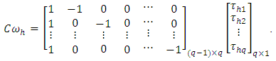 In the above,
  was the location-specific effect of treatment
  in the location
 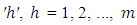 and
and  . Let
. Let  be a solution to the normal equations,
 Since
Since  were contrasts so they were estimable and the best linear unbiased estimate of
  were
were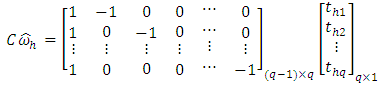 where,
  for
for  . For two ways interactions model,
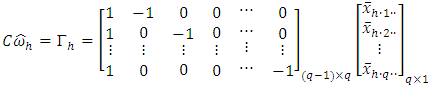 where,
  was the j-th (j = 1, 2, …,q) treatment mean of h-th (h= 1, 2, …,m) place.It was observed that
 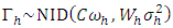 for h= 1, 2, …,p; where
  was a non-singular of
  order square matrix and was unique with respect to any choice of g-inverse
  of
of  . In practice
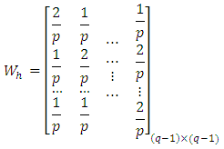 where, p was the number of blocks (replications) of the location specific experiment. Thus, for known
  , the suggested pooled test statistic for the null hypothesis (2.2) was given by
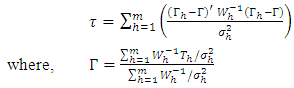 | (2.2) |
This test statistic (2.2) follow approximate χ2 distribution with (p–1)(q–1) d.f. when randomized block design or latin square design ( see, Ali et. al., 1999; Albassam and Ali, 2014) were consider for the experiments. The proof has been done in the same line of James (1954) and Albassam and Ali (2014). When  is unknown, then
  can be replaced by its usual unbiased estimate
  , i.e., mean sum square error of the model (2.1) in h-th location. We know
  are independently distributed as χ2 with fh (h = 1, 2, …, m) d.f. In our case,
  is the error mean sum of squares from h-th experiment and all error degrees of freedom
  are equal having value
  . Let
. Let  and
and  be the estimated values of τ and
  respectively after replacing
  by its estimate
  . Then, the test statistic (2.3) can be written as,
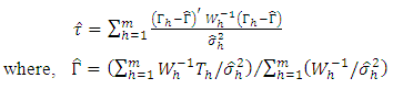 | (2.3) |
In view of James (1954) theorem it may be mention here that the statistic (2.3) may be follow χ2 distribution with 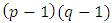 d.f. provided that
  are large. For
  not large enough, the statistic (2.3) may be compared with
 where
where 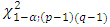 is the α% point of χ2-variate with
 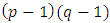 d.f. The test statistic (2.3) can be computed easily and provides the pooled estimate of treatment contrasts.The hypothesis (2.2) may be presented in another way. Assume that
  , for all h = 1, 2, …, m. Then, the hypothesis can be written as,H01:
  , against the alternative, H11:
  The test statistic is given by
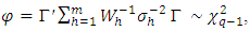 , if
, if  are known. If unknown
  were to be replaced by its estimates
  then the test statistic is given by
 Then
Then  under H01. For
  not large enough, the statistic
  is to be compared with
 where
where  is the α% point of χ2-variate with
  d.f. The hypothesis implies that all
  contrasts are insignificant. But it is sometimes required to test the insignificancy of any one of the contrasts. For this, the test statistic is given by,
 where
where  . The statistic
  provided
  are large. For
  not large enough,
  is to be compared with
 where,
  is the α% point of χ2-variate with
  d.f. In every case, James (1954) conjecture that the test statistic follow a χ2 distribution if
  are large, but there was no definite indication of the value of large
  . Thus, it was decided to study the distributional properties of the test statistic (2.3) for both small and moderately large values of
  using Monte Carlo simulation technique. For this, sets of random normal samples were drawn. In order to find the exact critical values of the statistic, a Monte Carlo study was performed. In this study, attempts were made to find the exact critical values, pdf, cdf and some other properties of the distribution of the test statistic (2.3) under the null hypothesis. These were calculated with eliminating outliers and without withdrawing the outliers from the series of the statistic (2.3).For eliminating lower and upper outliers, the formulae are
  and
and  where, FL = first quartile, FU = third quartile and dF = FU – FL. For a particular value of
  and for different values of
  sets of q (= 2, 3, 4, 5, …) normal observations were generated. A set of q observations for a particular value of
  have been considered as the observations of j-th treatment of p blocks. The set of q observations for different values of
  were considered the observations from a two ways interactions design. For different values of
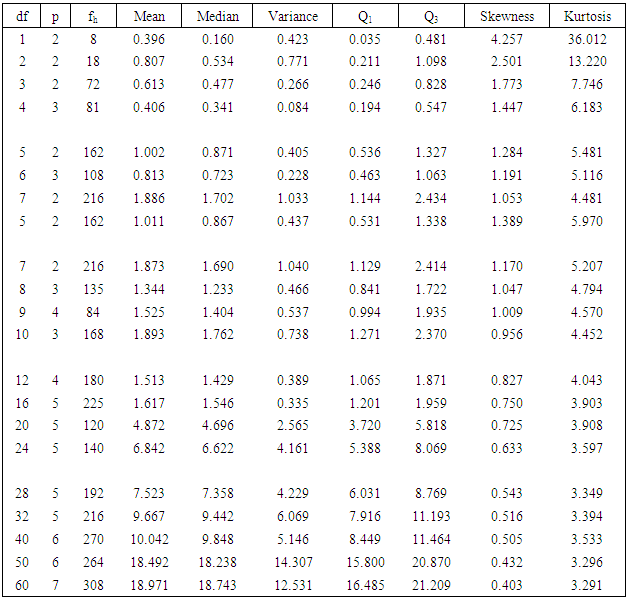
  (h = 1, 2, …, m), the observations of m two ways interaction designs were generated. The samples were generated to calculate the test statistic (2.3) under the null hypothesis. These processes were repeated 20,000 times and obtained 20,000 values of the test statistic (2.3). From these test statistic values, exact critical values corresponding to the nominal sizes 1%, 2%, 2.5%, 5%, 10%, 90%, 95%, 97.5%, 98%, 99% were calculated first from the original values and then eliminating outliers under the null hypothesis. Beside these, some other distributional characteristics such as mean, median, variance, skewness, kurtosis, empirical pdf and cdf were calculated for different df (degrees of freedom) of the test statistic. In each case, percentile points and other distributional characteristic were studied. Empirical fitted pdf and cdf curve of the distribution of the test statistic were also presented to observe the trend with the change of df of the statistic and error df of designs. For computer programming and simulation, MATLAB R2015a version was used.
3. Monte Carlo Study
In section 2, the derivation of the test statistic as well as the simulation procedure of obtaining percentile values, distributional characteristics, empirical fitted pdf and cdf curve of the test statistic (2.3) were discussed and they are presented in tabular form in this section.
3.1. Percentile Values
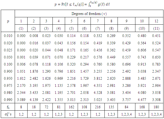
Simulated percentile values for the nominal sizes 1%, 2%, 2.5%, 5%, 10%, 90%, 95%, 97.5%, 98%, 99% are presented in to two tables and they are:Table 3.1: Simulated percentile points of the test statistic (2.3) under the null hypothesis.Table 3.1. Simulated percentile points of the test statistic (2.3) under H0
 |
| |
|
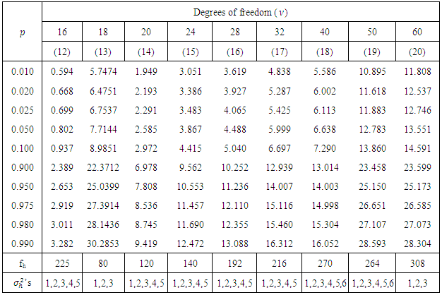
Table 3.1. (Continue)
 |
| |
|
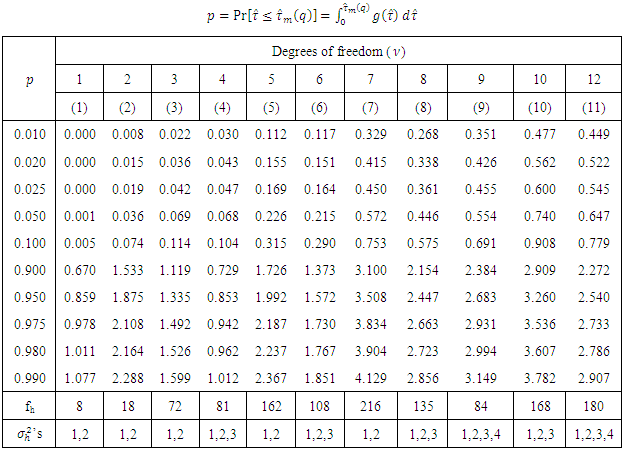
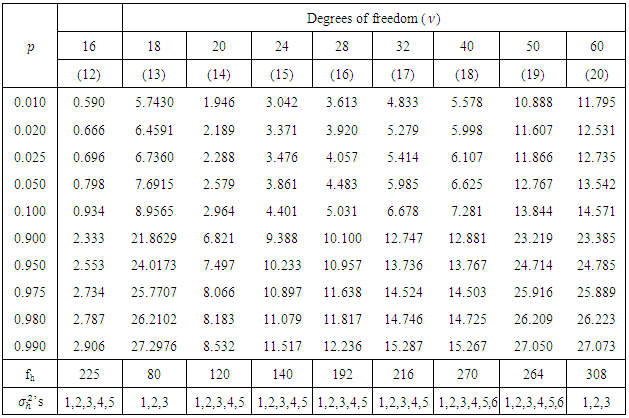
Table 3.2: Simulated percentile points of the test statistic (2.3) after elimination of outliers under the null hypothesis.Table 3.2. Simulated percentile points of the test statistic (2.3) after elimination of outliers under H0
 |
| |
|
Table 3.2. (Continue)
 |
| |
|
The entries of these tables are  , where,
  significance levels, p = 0.01, 0.02, 0.025, 0.05, 0.10, 0.90, 0.95, 0.975, 0.98, 0.99 and degrees of freedom (df),
  = 1, 2, 3, 4, 6, 8, 9, 10, 12, 16, 18, 20, 24, 28, 32, 40, 50, 60.
3.2. Distributional Characteristics
Further, a table indicating some distributional characteristics of the test statistic (2.3) is also presented in this section. This table includes mean, median, variance, skewness and kurtosis of the test statistic (2.3). This table will help to understand and unfold the properties of the test statistic (2.3). It will also help for preparation of a comparative study regarding the performance of the test statistic (2.3) and corresponding exact  test.
test.Table 3.3. Simulated distributional characteristics of the test statistic (2.3) under H0
 |
| |
|
4. Discussion and Interpretation
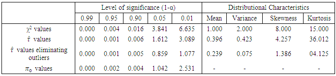
In view of AlBassam and Ali (2014), Jamjoom and Ali (2011) and Bhuyan (1986) based on James (1954) conjecture, the suggested test statistic (2.3) should be distributed as  when error degrees of freedom
  h = 1, 2, 3, …, m were large. But the critical values obtained from the simulated distribution of the test statistic differ significantly from those corresponding exact
  even for large error degrees of freedom. These may be observed by comparing the percentile points and the distributional characteristics of the test statistic (2.3) for different values of
  with those corresponding
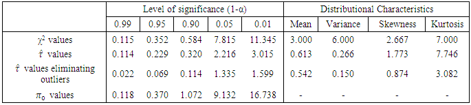
  -distribution. The following comparisons will make this point clear.From the below comparison (Table 4.1) it is observed that for 5% level of significance and for
  , the critical value of the simulated distribution is 1.612 (without eliminating outliers) and is 0.859 (with eliminating outliers). The corresponding value of
  -distribution is 3.841. Here, error degrees of freedom,
  , is small. Similar phenomenon was also observed by studying the mean, median, variance, skewness and kurtosis. However, James (1954) conjecture was to compare the calculated value of
  with the value of
  . But the 5% value of
  was significantly differ compare to the simulated 5% value of
  . This means that if the calculated value of
  lies between 0.859 (eliminating outliers) and 1.042 (=
 ) or 1.042 and 1.612 (without eliminating outliers), the researcher will wrongly accept or reject the null hypothesis of homogeneity of treatment contrasts. The conclusion of the researcher will not be disturbed in the case when calculated of
  will either be less than 0.859 or greater than 1.612. The percentile points at lower tail of the simulated distribution of the test statistic were however observed to be close to those corresponds of the exact
  -distribution and the corresponding value of
  . If we increase
  one step further the aforementioned problems remains more or less same. The following example will make it clear:
Table 4.1. df = 1, p = 2, fh = 8
 |
| |
|
Consider the moderately large error degrees of freedom of individual experiment, i.e.,  , the distribution
  will not follow the exact
  distribution. Of course the fact was also observed by studying the mean, median, variance, skewness and kurtosis of the distribution of
  . James (1954) conjecture was to compare the calculated value of
  with the value of
  . But the critical value of
  differ from the value of
  for different level of significance. The difference in the critical value of
  and in the value of
  increases with the decrease in the level of significance of the test. The value of
  and the critical value of
  were not same even for 90% level of significance. This means that the problem of test using the value of
  as critical value will not be obviated if the error degrees of freedom of individual experiments were increased still further. This may be observed from the following comparisons.
Table 4.2. df = 3, p = 2, fh = 72
 |
| |
|
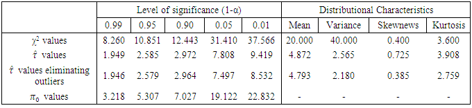
The below Table 4.3 represents the percentile points of the simulated distribution of  based on large error degrees of freedom. According to James (1954) conjecture this
  should be distributed as exact
  . But the mean, median, variance, skewness and kurtosis of
  do not support the James (1954) theory. The same was shown in the empirical pdf and cdf (from Fig 1 to Fig 18) of the test statistic
  (2.3). The percentile points of
  also differ with those of
  -distribution. This study thus indicates that the suggested test statistic (2.3) is not distributed as
  even for large error degrees of freedom will also be misleading. However, for valid conclusion using the statistic
  one can consult the percentile points of the simulated
  provided in this paper.
Table 4.3. df = 20, p = 5, fh = 120
 |
| |
|
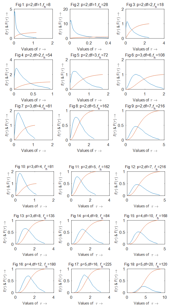 | Figure 4.1. Empirical probability density function (pdf) and cumulative distribution function (cdf) of test statistic  (2.3) for various df and error degrees of freedom fh (from Fig 1 to Fig 18) (2.3) for various df and error degrees of freedom fh (from Fig 1 to Fig 18) |
5. Application of the Method to Real Data Set
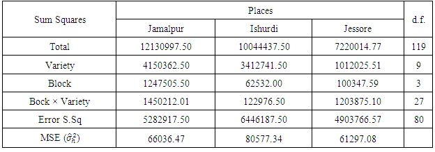
The data comes from a group of three experiments conducted for testing 10 varieties of wheat in three experimental places at i) Jamalpur, ii) Ishurdi, and ii) Jessore by Bangladesh Agricultural Research Institute (BARI) in Bangladesh in the year 1979-80. The experiments were conducted through two way interaction design in blocks of 40 plots each. In the experiments, N:P:K = 100:60:40 kg/ha was given as basal manure. The plot size was 4×5 meters and the yield in kg/ha was recorded.The object of the study was to test the significances of variety effects for all places. The analytical results of the three individual experiments are presented in Table 5.1.Table 5.1. ANOVA analysis of individual places
 |
| |
|
The estimates of treatment effects and the contrasts of the type th1-thj (h=1,2,3; j′ =2,3, ...,10) obtained from three individual places are presented in Table 5.2. Table 5.2. Estimates of treatments with their contrasts of individual places
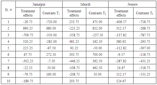 |
| |
|
Using estimated error variance  Bartlett’s (1937) χ2-test was performed and observed that the error variance were heterogeneous. Thus to test the significance of the treatment effects, the test statistic (2.3) was computed as
  = 18.246. According to James (1954) the statistic
  was to be compared with either the tabulated value of χ2 with (p-1)(q-1)=18 d.f. or with the critical value given by the statistic
  . The tabulated value,
 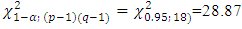 and
and  =29.081. The tabulated value based on the simulated distribution of
  is 7.6915 (from Table 3.2, coln. 13). From the analysis it was observed that the wheat variety contrasts were insignificant were as on the basis of the exact simulated percentile points of the statistic, the contrasts were observed as significant. In this case Jame’s (1954) suggestion distorted the conclusion on wheat variety effect.
6. Summary and Conclusions
The results obtained from the analysis of a single experiment, however accurate, can provide information only for a particular place or season and hence were not of much practical importance especially when the concern of the investigation becomes wider and more general in agricultural, industrial, scientific and medical fields. Thus the investigators were lead to repeat their experiments in heterogeneous environment over years/seasons or over centre’s/places to make more valid and realistic conclusion which may either cover a reasonably longer time span or a wider geographical area with heterogeneous agro-climatic and/or other important conditions. The objective of the investigators can be served better with usual combine analysis which is simple and straightforward in case of homogeneity of places/seasons. In the case when experiments were conducted over heterogeneous environment or over times/seasons with much varying characteristics the pooled analysis was complicated. The analysis becomes much more complicated if places significance with treatments interaction were observed in addition to the aforementioned heterogeneity of environments/seasons. In case of mixed effect heteroscedastic model, the presence of places with treatments interaction term makes the analysis a bit more complicated and in fact no exact test was possible even for known weights. Bhuyan (1984) and AlBassam and Ali (2014) in such a situation, suggested performing combined analysis of those treatments conducted in randomized block design and latin square design respectively whose were stable over places. This procedure was a bit lengthy and at the same time was not free of criticism. In this approach, individual experiments are conducted in two ways design model with interaction and a unified pooled test statistic is suggested to test treatment contrasts. According to James (1954) conjecture the suggested test statistic (2.3) will be distributed as an exact  -distribution if it is based on large error degrees of freedom. He however did not mention the limit of degrees of freedom beyond which one can consider it to be large. In this paper an attempt was made to find out exact critical values of the test statistic (2.3) through a Monte Carlo study for different parametric conditions. This was done under the null hypothesis in presence of outliers and after eliminating the outliers. Empirical pdf, cdf and some other distributional characteristics were also simulated and presented in this paper. From the Monte Carlo study, it is observed that the distribution of the statistic (2.3) was not distributed as
  even for large enough error degrees of freedom. The percentile points of the simulated distribution of the statistic differ significantly from those of corresponding
  -distribution and from James (1954) suggested approximate critical values
  for both small and large error degrees of freedom. As the convergence of the distribution of the test statistics (2.3) towards
  -distribution was not properly substantiated by the Monte Carlo study and the approximate critical values expressed in terms of the critical values of the exact
  -distribution were not vary to the exact critical values for small error degrees of freedom. Same also follows to the all distributional characteristics. It is very likely that the investigators will wrongly reject or accept the null hypothesis if they take decision on the basis of those approximate critical values. This fact was observed in practical problems. However for valid inference using the statistic
  one should be more careful and may consult the simulated critical values of the distribution of the statistic
  embodied in this paper.
ACKNOWLEDGEMENTS
Authors are grateful to the reviewer for his fruitful suggestions which enrich the paper.
References
| [1] | AlBassam, M.S. and Ali, M.A. (2014). Test statistic for combined treatment contrast under heterogeneous error variances and Latin square design. Pakistan J. Statist. Vol. 30(3), 345-360. |
| [2] | Bhuyan, K.C. (1984). A group of split-split-plot designs with a heterogeneous model. Aust. J. Statist., 26(2), 132-141. |
| [3] | Bhuyan, K.C. (1986). A method of intra-block analysis of a group of BIB deigns with heterogeneous error variances. Gujrat Statistical Review, XIII(1), 1986. |
| [4] | Aiken, L.S. and West, S.G. (1991). Multiple Regression: Testing and interpreting interactions. Newbury Park, London, Sage. |
| [5] | Blouin, D.C., Webster, E.P. and Bond, J.A. (2011). On the analysis of combined experiments Weed Technology, 25(1), 165-169. |
| [6] | Cochran, W.G. (1937). Problems arising in the analysis of a series of similar experiments, J. Roy. Statist. Soc. Supp., 4, 102-118. |
| [7] | Cochran, W.G. (1954). The combination of estimates from different experiments. Biometrics, 10, 101-129. |
| [8] | Danbaba, A and Shehu, A. (2016). On the combined analysis of sudoku square designs with some common treatments. Int. J. Statist. Appli. Vol. 6(6), 347-351. |
| [9] | Dawson, J.F. (2014). Moderation in management research: What, why when and how. J. of Busi. and Psy., 29, 1-19. |
| [10] | Gomes, F.P. and Guimaraes, R.F. (1958). Joint analysis of experiments incomplete randomized blocks with some common treatments. Biometrics, 14, 521-526. |
| [11] | James, G.S. (1951). The comparison of several groups of observations when the ratios of the population variances are unknown. Biometrika, 33, 324-329. |
| [12] | James, G.S. (1954). Test of linear hypothesis in univariate analysis when the ratios of the population variances are unknown. Biometrika, 41, 19-43. |
| [13] | Jamjoom, A.A. and Ali, M.A. (2011). Pooled test statistic of treatment contrast and randomized block design with heterogeneous environment. Alig. J. Statist., 31, 63-79. |
| [14] | Moore, K.J. and Dixon, P.M. (2015). Analysis of combined experiments revisited. Agronomy Journal. Vol 107(2), 763-771. |

 Abstract
 Reference
 Full-Text PDF
 Full-text HTML