1. Introduction

In public health and in applied research in general, analysts frequently use automated variable selection methods such as backward elimination or forward selection in order to identify independent predictors of an outcome or for developing parsimonious regression models [1-3]. Automatic variable selection methods in regression results in spurious noise variables being mistakenly identified as independent predictors of the outcome [4, 5]. Furthermore, the use of these methods can result in the selection of non-reproducible regression models [6] with the p-values and estimated standard errors of regression coefficients biased downwards and regression coefficients biased further away from zero resulting in stronger associations than actually is [7]. Despite these methodological problems, automated methods continue to be used unabatedly in various areas of public health and medical research. The popularity of automated techniques have arisen because they are discussed in nearly all elementary textbooks on applied statistics and implemented in almost all commercial statistical software packages. Although there are some methods for correcting p values for forward selection [8] and a range of automated variable selection methods [9], they are not yet directly available in any software for users to correct their p values. Also, these methods do not provide corrections for effect sizes. So, the analysts who are using automated methods for variable selection cannot correct their p values and effect sizes without doing programming. This means they need to be very cautious while interpreting the results for their variable selection. The analysts need to at least compare the variables selected by automated methods to a variable selection method which is likely to select the true predictors of an outcome, and assess overfitting (selecting more predictors than there actually is) and overestimation in effect size.

In this article, we assess the performance of epidemiologic logistic regression models selected by automated variable selection against models selected by forced entry using multiple bootstrap samples. The latter variable selection method is not novel. In fact, Harrell in 2002 [10] showed the use of simple bootstrap methods for variable selection. Harshman and Lundy [11] and Freedman et al. [12] also thought that simple bootstrapping may be a solution. This method is relatively simple compared to existing shrinkage and machine learning methods for variable selection and is therefore easier for clinicians and medical practitioners to grasp, however, its practical implementation in a computer software remains unavailable. To facilitate the practical application of the given method we provide computer programs (SAS macros) using examples from cardiovascular disease risk prediction. The SAS macros given in this article can be adapted for outcomes other than CVD incidence as required by the user. It is not the aim of the current paper to compare the performance of the given bootstrap method against existing shrinkage and machine learning methods. This could be the scope for another paper. The intended audience for this article are those who are using automated variable selection methods and would like to continue doing so in future despite its various shortcomings.

For automated variable selection, we apply the most commonly used methods, namely, forward selection, backward elimination and stepwise selection. We compare the significant predictors selected by automated variable selection to the significant predictors which occur more than half the times by forced entry based on 1000 bootstrap samples. This would enable us to detect any evidence of overfitting. We also compare the effect size or odds ratio of the significant predictors selected by automated variable selection to the average effect size or odds ratio of these predictors obtained from fitting the same regression model by forced entry using 1000 bootstrap samples. This will indicate the extent of overestimation or underestimation in the effect size for the significant predictors selected by automated variable selection. To check for the stability of our bootstrap regression approach, we examine the direction of all regression coefficients. If they are either all positive or all negative then it can be an indication of stability of our bootstrap regression approach as has been suggested by Austin and Tu [13].

1.1. Shrinkage and Machine Learning Methods for Variable Selection

Over the past decade, there has been a tremendous amount of research into the use of shrinkage and machine learning approaches for selecting variables in prognostic models. In this section, we very briefly review these methods.

The lasso or Least Absolute Shrinkage and Selection Operator [14] type models have become popular methods for variable selection when there are many predictors analyzed due to their property of shrinking variables with very unstable estimates to exactly zero. By shrinking to zero, the LASSO model can effectively exclude some irrelevant variables and produce sparse estimations. Theory states that lasso type methods are able to do consistent variable selection, but it is hard to achieve this property in practice. In practice, the LASSO model creates excessive biases when selecting significant variables and is not consistent in terms of variable selection [15, 16]. This consistent variable selection highly depends on the right choice of the tuning parameter. This can only be obtained under certain conditions [17, 18]. The second reference is in the context of epidemiological association studies.

Variable selection by machine learning models has become the focus of much research in areas of application for which datasets with tens or hundreds of thousands of variables are available. The machine learning models not only find main effects variables, but interactions between variables and subsets of variables. There are three main categories of variable selection in machine learning:

(i) Filter: These methods search for significant variables by looking at the characteristics of each individual variable using an independent test such as the information entropy and statistical dependence test. Following the classification of Kohavi and John [19], variable ranking is a filter method and is a pre-processing step which is independent of the choice of the predictor.

(ii) Wrapper or embedded method: These methods apply a specific machine learning algorithm such as the decision tree or support vector machine or linear discriminant analysis (LDA) or a multi-class version of Fisher’s linear discriminant [20] or multi-class SVMs (see, e.g., Weston et al. [21]) and utilizes the corresponding classification performance to guide the variable selection. These methods depend upon the capability of the classifier used to handle the multi-class case.

(iii) Hybrid methods: These combine the advantages of filter and wrapper methods.

Details of machine learning methods for variable selection are described elsewhere [22].

1.2. Methods for Correcting P Values for Automated Variable Selection

We mainly discuss here methods which provide closed form solutions for corrected p values. One method is a recent development by Taylor and Tibshirani [8] which provides selection-adjusted p values for forward variable selection. Brombin et al. [9] has proposed a nonparametric permutation solution that is exact, flexible and potentially adaptable to most types of automated variable selection. The correction becomes more severe when many variables are processed by the stepwise machinery. There are also sampling based methods under development, using Markov-chain Monte Carlo and bootstrapping, that can provide improvements in power [23].

1.3. Bootstrap Methods for Variable Selection

In the well-known bootstrapping method, bootstrap samples of the same size as the original sample are drawn with replacement from the original sample, reflecting the drawing of samples from an underlying population. In an attempt to select variables for a multiple logistic regression, Austin and Tu [13] proposed a model selection method based upon using backward elimination in multiple bootstrap samples. An empirical examination of this method found that it does not perform better than standard backward elimination [24]. This implies that backward elimination incorporating bootstrapping does not improve model selection compared to standard backward elimination.

Harrell [7] has exhibited how bootstrap methods can be used for variable selection. This included simple bootstrapping and bootstrapping incorporating automated methods. Since the latter does not improve variable selection which we have discussed above [24], we implement in this article a simple and practical implementation of simple bootstrapping for variable selection.

2. Methods

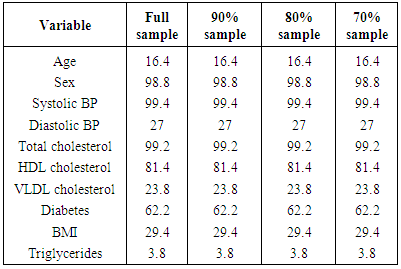
Forced entry regression using multiple bootstrap samples is implemented through several steps. First, a model is constructed in the original sample by selecting predictors from a larger set of candidate predictors using an automated variable selection method. Then this model is compared to the model selected by forced entry using bootstrap samples. With a bootstrap regression, first a specific model is repeatedly fitted using each bootstrap sample. Bootstrapping is used to assess the distribution of an indicator variable denoting the statistical significance of a specific predictor variable in a model where all candidate predictors were initially selected by univariate regression and found to have no collinearity problems. One would expect that variables that truly were independent predictors of the outcome would be identified as independent predictors by forced entry in a majority of the bootstrap samples, while noise variables would be identified as independent predictors in only a minority of samples. This approach has also been discussed by Harrell [10]. Using the results of the bootstrap sampling, we created a series of candidate models for predicting CVD incidence. They contained the variables that were selected in 100%, 90%, 80% and 70% of the bootstrap samples using forced entry logistic regression. The use of both the full sample and sub-samples to implement the bootstrap regression models helped to assess their stability. This approach was used by Austin and Tu [13] for assessing the stability of significant predictors selected by automated variable selection for logistic regression. The methodology is discussed in detail by Harrell [10].

For building a multivariate logistic regression model for predicting the occurrence of a CVD event, we considered a list of 12 sociodemographic, dietary and laboratory risk factors, namely, age (in years), sex (0=male, 1=female), low calorie diet, low fat diet, VLDL cholesterol, HDL cholesterol, total cholesterol, diabetes (0=no, 1=yes), systolic blood pressure, diastolic blood pressure, triglycerides and body mass index.

2.1. Datasets Used

The data used for our epidemiologic model building was a subset of the sample drawn from Framingham Heart Study (FHS). The FHS was established in 1948 that followed a cohort of 5209 adults from Framingham, Massachusetts, to examine the relationship between health risk factors and subsequent CVD. Although we will not use it in this study, a further 5124 people who were offspring of the original participants joined the original cohort in 1971 and were known as the ‘offspring cohort’. This provides the only health data which allow very long-term regular follow-up of participants with health examinations conducted by health professionals and with enough study participants to provide the statistical power to examine detailed epidemiological hypotheses. The design, selection criteria and examination procedures of FHS have previously been elaborated in detail [25-29]. The outcome of interest is the occurrence of first CVD which includes stroke, myocardial infarction, angina pectoris, coronary insufficiency and sudden death. The study cohort consisted of people from examination 1 (1971–1975) of the offspring cohort and from examinations 10 and 11 (1968–1971) of the original cohort for whom high-density lipoprotein (HDL) cholesterol levels were measured for the first time. For the original cohort, in most cases (81.3%), HDL was measured for the first time at examination 11, while for some cohort members, it was examination 10. Follow-up was performed through the 22nd examination cycle, a span of approximately 24 years. For the offspring cohort, risk factor measurements were from the first examination cycle (1971–1975), whereas follow-up was performed through the sixth examination cycle, approximately 24 years later. Participants were considered eligible if at the baseline they were aged 30–49 years, were free of CVD (CHD and stroke), and had complete information on covariates. After exclusions, the study included 964 persons (493 events, 471 non-events).

3. Results

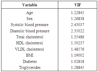
The results of univariate logistic regression analysis are presented in Table 1. These indicate that 10 out of 12 potential predictors are statistically significant at 25% level of significance. These are: age, sex, systolic blood pressure, diastolic blood pressure, HDL cholesterol, VLDL cholesterol, total cholesterol, triglycerides, diabetes and body mass index.

Table 1. The p-values of candidate predictors based on univariate logistic regression analysis

There was no evidence of any significant collinearity as the variance inflation factor did not exceed 10 for any of the potential predictors. This is demonstrated in Table 2.

Table 2. Variance inflation factor of the candidate predictors selected by univariate logistic regression

For multivariate logistic regression analysis, the variables which were found to be independent predictors of the outcome by the three automated variable selection methods are summarised as follows. Backward elimination variable selection identified five significant predictors, namely, sex, systolic blood pressure, total cholesterol, HDL cholesterol and diabetes. Forward variable selection identified five significant predictors, namely, sex, systolic blood pressure, total cholesterol, HDL cholesterol and VLDL cholesterol. Stepwise variable selection identified five significant predictors, namely, sex, systolic blood pressure, total cholesterol, HDL cholesterol and diabetes.

Based on forced entry logistic regression using 1000 bootstrap samples selected from the full observed sample, the most commonly occurring (more than 50% times) significant predictors are systolic blood pressure (99.4% times), total cholesterol (99.2% times), sex (98.8% times), HDL cholesterol (81.4% times) and diabetes (62.2% times). These results are unchanged for 90%, 80% and 70% subsamples. These are summarised in Table 3. Comparing these results to those by automated variable selection we see that forward selection includes a noise predictor, namely, VLDL cholesterol. It is a noise predictor since it is found to be a significant predictor less than 50% times (23.8% based on 100%, 90%, 80% and 70% samples) by forced entry bootstrapping. Backward elimination and stepwise variable selection do not select any noise predictor.

Table 3. Relative frequency (%) with which each candidate variable was selected using forced entry model selection in 1000 bootstrap samples drawn from the Framingham original cohort

The effect size in terms of odds ratios of the significant predictors selected by automated variable selection clearly indicates evidence of overestimation. This is more prominent for diabetes and sex which are categorical variables. The degree of overestimation seems to be higher for forward variable selection compared to the other two automated variable selection methods. Between backward elimination and stepwise variable selection, there is no difference in the degree of overestimation. These results are presented in Table 4.

Table 4. Estimates of relative odds for each selected independent predictor by automated variable selection methods and the proposed bootstrap regression approach

The signs of all bootstrap regression coefficients are shown in Table 5. The results show that all bootstrap regression coefficients are either all positive or all negative. This is an indication of stability of our bootstrap regression approach.

Table 5. Distribution of signs of all bootstrap regression coefficients for the true predictors selected by the proposed bootstrap regression approach

4. Conclusions

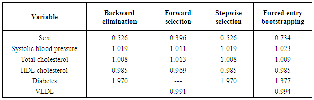
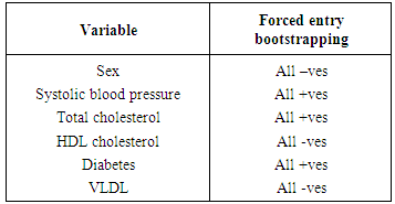
The importance of using theory in choosing variables whenever available has long been a practice in many practical applications of regression models. However, in situations when they are unavailable automated variable selection methods have been very popular. These fields include public health and medical research among others. However, automated variable selection methods have been widely criticised by statisticians due to various methodological reasons. The criticisms include producing downwardly biased p-values (overfitting), overestimating regression coefficients as well as effect sizes and producing narrower confidence intervals than they actually are. Despite these methodological problems, automated methods continue to be used unabatedly in various areas of public health and medical research. The methods for correcting the p values for an automated variable selection method are not directly available in softwares. So, the analysts need to be very cautious while using automated methods for variable selection. The analysts need to at least compare the results of automated methods to a variable selection method which is likely to select the true predictors of an outcome. This will assist them greatly to identify any noise predictor selected by automated methods. If analysts report the regression coefficients and/or effect sizes of the predictors selected by automated methods, then they need to assess the degree of bias in the regression coefficients and/or effect sizes obtained by automated methods. To provide these we discuss a bootstrapping based regression approach discussed by Harrell [7] in which a specific model is repeatedly fitted using each bootstrap sample in order to assess the distribution of an indicator variable denoting the statistical significance of a specific predictor variable in a model where all candidate predictors were initially selected by univariate regression and found to have no collinearity problems. One would expect that variables that truly were independent predictors of the outcome would be identified as independent predictors by forced entry in a majority of the bootstrap samples, while noise variables would be identified as independent predictors in only a minority of samples. Using data from the well-known Framingham heart study we provide an example of variable selection for logistic regression when the outcome is the occurrence of an incident cardiovascular event. We apply the most commonly used automated variable selection methods, namely, forward selection, backward elimination and stepwise selection. We compare the significant predictors selected by automated variable selection to the significant predictors which occur more than half the times by forced entry based on 1000 bootstrap samples. We also compare the effect size of the significant predictors selected by automated variable selection to the average effect size of these predictors obtained from fitting the same regression model using 1000 bootstrap samples. We provide in the appendix the required programming codes to conduct these analyses using the SAS software.

The results showed that a noise predictor (VLDL cholesterol) was selected by forward variable selection while neither backward elimination nor stepwise variable selection selected any noise predictor. However, in our case study the number of candidate predictors was only 10 which resulted in the selection of such a small number of noise predictors. It has been shown that for automated variable selection the number of noise predictors included increases as the number of candidate variables increases, and the probability of correctly identifying variables is inversely proportional to the number of variables under consideration [30].

There was clear evidence of overestimation in regression coefficients and effect sizes for the independent predictors selected by automated methods. The degree of overestimation was higher for forward variable selection compared to the other two automated variable selection methods. Between backward elimination and stepwise variable selection, there was no difference in the degree of overestimation. Given our SAS codes, one can easily estimate the degree of overestimation in odds ratios for assessing the degree of accuracy in effect sizes for independent predictors selected by automated variable selection methods.

The primary advantage of our proposed variable selection method is that it allows one to assess the stability of independent predictors and their estimated regression coefficients selected by automated methods. For a given predictor variable, one can examine the distribution of the associated regression coefficient across the bootstrap samples. We found that the bootstrap regression coefficients were either all positive or all negative (SAS macros given in appendix). This demonstrated the stability of our approach. On the contrary, the approach suggested by Austin and Tu [13] may select a somewhat unstable model if a variable was selected as an independent predictor in a majority of bootstrap samples while some estimated coefficients were positive and some negative. This approach will select a totally unstable model in rare situations when half the estimated coefficients were positive and half were negative. Another advantage of our approach is that initial screening out of variables with high multicollinearity prior to inclusion of variables in our bootstrap regression approach ensured that the bootstrap regression coefficients were stable in terms of precision or standard error. Our approach can also be used to examine models with interactions or higher order terms. In that case one could use our proposed model selection method to derive a model of main effects, and then explore the presence of interactions and higher order terms.

Finally, the SAS macros provided at the end of this paper in appendices 1a through 1g are easy to follow and implement and can be easily adapted to different datasets involving a range of predictors and a binary outcome variable when the primary interest is to select independent predictors and/or assess the magnitude of the effect size of these independent predictors arising from logistic regression analysis. For other types of common outcome variables, for instance, continuous and time to event data, one can replace proc logistic by the appropriate regression procedure in SAS and still adapt our codes to perform the analysis.

ACKNOWLEDGEMENTS

We acknowledge the use of public use datasets for Framingham heart study which are anonymized, freely available datasets for research purposes. The link for this website is available from: https://biolincc.nhlbi.nih.gov/teaching/.

Appendix

Appendix 1a: SAS codes for univariate logistic regression of CVD incidence

Proc logistic data=OUTDAT.FULL_FOLLOW_UP

desc;

Class sex/ref=first; /*for sex, 0=male, 1=female*/

Model cvdflg=sex;

Proc logistic data=OUTDAT.FULL_FOLLOW_UP

desc;

Class diab/ref=first; /*for diabetes, 0=no, 1=yes*/

Model cvdflg=diab;

Proc logistic data=OUTDAT.FULL_FOLLOW_UP

desc;

Model cvdflg=ageyr;

Proc logistic data=OUTDAT.FULL_FOLLOW_UP

desc;

Model cvdflg=sbp;

Proc logistic data=OUTDAT.FULL_FOLLOW_UP

desc;

Model cvdflg=dbp;

Proc logistic data=OUTDAT.FULL_FOLLOW_UP desc;

Model cvdflg=totchol;

Proc logistic data=OUTDAT.FULL_FOLLOW_UP desc;

Model cvdflg=hdl;

Proc logistic data=OUTDAT.FULL_FOLLOW_UP desc;

Model cvdflg=bmi ;

Proc logistic data=OUTDAT.FULL_FOLLOW_UP desc;

Model cvdflg=fd38;

Proc logistic data=OUTDAT.FULL_FOLLOW_UP desc;

Model cvdflg=fc32;

run;

Appendix 1b: SAS codes for checking collinearity

Proc logistic data=OUTDAT.FULL_FOLLOW_UP desc;

Class sex diab/ref=first;

Model cvdflg=ageyr sex sbp dbp totchol hdl bmi diab vldl trig;

output out=pred pred=p;

data a;

set pred;

wt=p*(1-p);

run;

proc reg data=a;

model cvdflg=ageyr sex sbp dbp totchol hdl bmi diab vldl trig/vif;

weight wt;

run;

Appendix 1c: SAS codes for selection of independent predictors of CVD incidence by automated variable selection

Proc logistic data=OUTDAT.FULL_FOLLOW_UP desc;

Class sex diab/ref=first;

Model cvdflg=ageyr sex sbp dbp totchol hdl bmi diab vldl trig/selection=forward;

Proc logistic data=OUTDAT.FULL_FOLLOW_UP desc;

Class sex diab/ref=first;

Model cvdflg=ageyr sex sbp dbp totchol hdl bmi diab vldl trig/selection=backward;

Proc logistic data=OUTDAT.FULL_FOLLOW_UP desc;

Class sex diab/ref=first;

Model cvdflg=ageyr sex sbp dbp totchol hdl bmi diab vldl trig/selection=stepwise;

run;

Appendix 1d: SAS macro for determining the frequency and relative frequency of independent predictors using the proposed forced entry bootstrapping approach

%macro boot;

%do i=1 %to 500; /* Create independent sets of replications */

data boot;

choice=int(ranuni(23456+&i)*n)+1;

set outdat.full_follow_up nobs=n point=choice;

j+1;

if j>n then stop;

run;

Ods exclude ParameterEstimates;

Proc logistic data=boot desc;

Class sex diab/ref=first;

Model cvdflg=ageyr sex sbp dbp totchol hdl bmi diab vldl trig;

ods output ParameterEstimates = est;

data wald (keep=pid variable waldchisq estimate);

set est;

pid=_n_;

run;

Proc transpose data=wald out=wide prefix= waldchisq;

By pid; /*identifier*/

var waldchisq;

id variable;

run;

data boot&i;

set wide;

array covs{10} waldchisqageyr waldchisqsex waldchisqsbp waldchisqdbp waldchisqtotchol waldchisqhdl waldchisqbmi waldchisqdiab waldchisqvldl waldchisqtrig;

array sigcov{10} sage&i ssex&i ssbp&i sdbp&i stchol&i shdl&i sbmi&i sdiab&i svldl&i strig&i;

do k=1 to 10;

sigcov{k}=0;

If covs{k}>=3.84 then sigcov{k}=1;

end;

id=_n_;

run;

proc sort data=boot&i; by id; run;

%end; /* end of bootstrapping loop*/

data comb;

merge boot1-boot500;

by id;

run;

proc means data=comb noprint;

var sage1-sage500 ssex1-ssex500 ssbp1-ssbp500 sdbp1-sdbp500 stchol1-stchol500 shdl1-shdl500 sbmi1-sbmi500 sdiab1-sdiab500 svldl1-svldl500 strig1-strig500;

output out=vsum sum= sage1-sage500 ssex1-ssex500 ssbp1-ssbp500 sdbp1-sdbp500 stchol1-stchol500 shdl1-shdl500 sbmi1-sbmi500 sdiab1-sdiab500 svldl1-svldl500 strig1-strig500;

run;

data total;

set vsum;

fvar1=sum(of sage1-sage500);

fvar2=sum(of ssex1-ssex500);

fvar3=sum(of ssbp1-ssbp500);

fvar4=sum(of sdbp1-sdbp500);

fvar5=sum(of stchol1-stchol500);

fvar6=sum(of shdl1-shdl500);

fvar7=sum(of sbmi1-sbmi500);

fvar8=sum(of sdiab1-sdiab500);

fvar9=sum(of svldl1-svldl500);

fvar10=sum(of strig1-strig500);

rename fvar1=fage fvar2=fsex fvar3=fsbp fvar4=fdbp fvar5=ftchol fvar6=fhdl fvar7=fbmi fvar8=fdiab fvar9=fvldl fvar10=ftrig;

array fcov{10} fvar1-fvar10;

array rfcov{10} rfvar1-rfvar10;

do l=1 to 10;

rfcov{l}=100*(fcov{l}/500);

end;

rename rfvar1=rfage rfvar2=rfsex rfvar3=rfsbp rfvar4=rfdbp rfvar5=rftchol rfvar6=rfhdl rfvar7=rfbmi rfvar8=rfdiab rfvar9=rfvldl rfvar10=rftrig;

run;

proc print; var fage rfage fsex rfsex fsbp rfsbp fdbp rfdbp ftchol rftchol fhdl rfhdl fbmi rfbmi fdiab rfdiab fvldl rfvldl ftrig rftrig;

run;

%mend boot;

%boot

Appendix 1e: SAS macro for determining the frequency and relative frequency of independent predictors using the proposed forced entry bootstrapping approach based on a subsample

/* Analysis here is based on 90% subsample. For analyses based on 80% & 70% subsamples the codes are identical except that 0.9 should be replaced by the appropriate value which is shown in the comment below*/

%macro boot_subsample;

%do i=1 %to 500; /* Create independent sets of replications */

data sub;

set outdat.full_follow_up;

random=ranuni(23457);

run;

proc sort; by random;

data sub;

set sub;

if random<=0.9; /* Here 0.9 should be replaced by 0.8 or 0.7 for 80% subsample or 70% subsample, respectively*/

run;

data boot;

choice=int(ranuni(23456+&i)*n)+1;

set sub nobs=n point=choice;

j+1;

if j>n then stop;

run;

Ods exclude ParameterEstimates;

Proc logistic data=boot desc;

Class sex diab /ref=first;

Model cvdflg=ageyr sex sbp dbp totchol hdl bmi diab vldl trig;

ods output ParameterEstimates = est;

data wald (keep=pid variable waldchisq estimate);

set est;

pid=_n_;

run;

Proc transpose data=wald out=wide prefix= waldchisq;

By pid; /*identifier*/

var waldchisq;

id variable;

run;

data boot&i;

set wide;

array covs{10} waldchisqageyr waldchisqsex waldchisqsbp waldchisqdbp waldchisqtotchol waldchisqhdl waldchisqbmi waldchisqdiab

waldchisqvldl waldchisqtrig;

array sigcov{10} sage&i ssex&i ssbp&i sdbp&i stchol&i shdl&i sbmi&i sdiab&i svldl&i strig&i;

do k=1 to 10;

sigcov{k}=0;

If covs{k}>=3.84 then sigcov{k}=1;

end;

id=_n_;

run;

proc sort data=boot&i; by id; run;

%end; /* end of bootstrapping loop*/

data comb;

merge boot1-boot500;

by id;

run;

proc means data=comb noprint;

var sage1-sage500 ssex1-ssex500 ssbp1-ssbp500 sdbp1-sdbp500 stchol1-stchol500 shdl1-shdl500 sbmi1-sbmi500 sdiab1-sdiab500 svldl1-svldl500 strig1-strig500;

output out=vsum sum= sage1-sage500 ssex1-ssex500 ssbp1-ssbp500 sdbp1-sdbp500 stchol1-stchol500 shdl1-shdl500 sbmi1-sbmi500 sdiab1-sdiab500 svldl1-svldl500 strig1-strig500;

run;

data total;

set vsum;

fvar1=sum(of sage1-sage500);

fvar2=sum(of ssex1-ssex500);

fvar3=sum(of ssbp1-ssbp500);

fvar4=sum(of sdbp1-sdbp500);

fvar5=sum(of stchol1-stchol500);

fvar6=sum(of shdl1-shdl500);

fvar7=sum(of sbmi1-sbmi500);

fvar8=sum(of sdiab1-sdiab500);

fvar9=sum(of svldl1-svldl500);

fvar10=sum(of strig1-strig500);

rename fvar1=fage fvar2=fsex fvar3=fsbp fvar4=fdbp fvar5=ftchol fvar6=fhdl fvar7=fbmi fvar8=fdiab fvar9=fvldl fvar10=ftrig;

array fcov{10} fvar1-fvar10;

array rfcov{10} rfvar1-rfvar10;

do l=1 to 10;

rfcov{l}=100*(fcov{l}/500);

end;

rename rfvar1=rfage rfvar2=rfsex rfvar3=rfsbp rfvar4=rfdbp rfvar5=rftchol rfvar6=rfhdl rfvar7=rfbmi rfvar8=rfdiab rfvar9=rfvldl rfvar10=rftrig;

run;

proc print; var fage rfage fsex rfsex fsbp rfsbp fdbp rfdbp ftchol rftchol fhdl rfhdl fbmi rfbmi fdiab rfdiab fvldl rfvldl ftrig rftrig;

run;

%mend boot_subsample;

%boot_subsample

Appendix 1f: SAS macro followed by required codes for calculating average (mean or median as appropriate) effect sizes

%macro boot2;

%do i=1 %to 500; /* Create independent sets of replications */

data boot;

choice=int(ranuni(23456+&i)*n)+1;

set outdat.full_follow_up nobs=n point=choice;

j+1;

if j>n then stop;

run;

Ods exclude ParameterEstimates;

Proc logistic data=boot desc;

Class sex diab/ref=first;

Model cvdflg=ageyr sex sbp dbp totchol hdl bmi diab vldl trig;

ods output ParameterEstimates = est;

data a(keep=pid variable estimate odds);

set est;

odds=exp(estimate);

pid=_n_;

run;

Proc transpose data=a out=wide prefix= odds;

By pid; /*identifier*/

var odds;

id variable;

run;

data boot&i;

set wide;

array ocovs{10} oddsageyr oddssex oddssbp oddsdbp oddstotchol oddshdl oddsbmi oddsdiab oddsvldl oddstrig;

do k=1 to 10;

odds&i=ocovs{k};

output;

end;

id=_n_;

run;

proc sort data=boot&i; by id; run;

%end; /* end of bootstrapping loop*/

data comb;

merge boot1-boot500;

by id;

mean_oddsratio=mean(of odds1-odds500);

median_oddsratio=median(of odds1-odds500);

if mean_oddsratio>.;

if median_oddsratio>.;

diff_oddsratio=mean_oddsratio-median_oddsratio;

if diff_oddsratio eq 0 then oddsratio=mean_oddsratio;

else if diff_oddsratio ne 0 then oddsratio=median_oddsratio;

run;

data comb;

set comb;

id=_n_;

run;

proc sort data=comb;

by id;

%mend boot2;

%boot2

data var;

input id variable $;

cards;

1 ageyr

2 sex

3 sbp

4 dbp

5 totchol

6 hdl

7 bmi

8 diab

9 vldl

10 trig

;

run;

proc sort data=var;

by id;

data final;

merge comb var;

by id;

proc print data=final;

var variable mean_oddsratio median_oddsratio oddsratio;

run;

Appendix 1g: SAS macro for calculating relative frequency of positive or negative effects

%macro boot3;

%do i=1 %to 500; /* Create independent sets of replications */

data boot;

choice=int(ranuni(23456+&i)*n)+1;

set outdat.full_follow_up nobs=n point=choice;

j+1;

if j>n then stop;

run;

Ods exclude ParameterEstimates;

Proc logistic data=boot desc;

Class sex diab/ref=first;

Model cvdflg=ageyr sex sbp dbp totchol hdl bmi diab vldl trig;

ods output ParameterEstimates = est;

data wald (keep=pid variable waldchisq estimate);

set est;

pid=_n_;

run;

Proc transpose data=a out=wide prefix= estimate;

By pid; /*identifier*/

var estimate;

id variable;

run;

data boot&i;

set wide;

array ecovs{10} estimateageyr estimatesex estimatesbp estimatedbp estimatetotchol estimatehdl estimatebmi estimatediab estimatevldl estimatetrig;

array poseff{10} eage&i esex&i esbp&i edbp&i etchol&i ehdl&i ebmi&i ediab&i evldl&i etrig&i;

do k=1 to 10;

poseff{k}=0;

If ecovs{k}>=0 then poseff{k}=1;

end;

id=_n_;

run;

proc sort data=boot&i; by id; run;

%end; /* end of bootstrapping loop*/

data comb;

merge boot1-boot500;

by id;

run;

proc means data=comb noprint;

var eage1-eage500 esex1-esex500 esbp1-esbp500 edbp1-edbp500 etchol1-etchol500 ehdl1-ehdl500 ebmi1-ebmi500 ediab1-ediab500 evldl1-evldl500 etrig1-etrig500;

output out=vsum sum= eage1-eage500 esex1-esex500 esbp1-esbp500 edbp1-edbp500 etchol1-etchol500 ehdl1-ehdl500 ebmi1-ebmi500 ediab1-ediab500

evldl1-evldl500 etrig1-etrig500;

run;

data total;

set vsum;

evar1=sum(of eage1-eage500);

evar2=sum(of esex1-esex500);

evar3=sum(of esbp1-esbp500);

evar4=sum(of edbp1-edbp500);

evar5=sum(of etchol1-etchol500);

evar6=sum(of ehdl1-ehdl500);

evar7=sum(of ebmi1-ebmi500);

evar8=sum(of ediab1-ediab500);

evar9=sum(of evldl1-evldl500);

evar10=sum(of etrig1-etrig500);

rename evar1=eage evar2=esex evar3=esbp evar4=edbp evar5=etchol evar6=ehdl evar7=ebmi evar8=ediab evar9=evldl evar10=etrig;

array fecov{10} evar1-evar10;

array rfecov{10} rfevar1-rfevar10;

do l=1 to 10;

rfecov{l}=100*(fecov{l}/500);

end;

rename rfevar1=rfeage rfevar2=rfesex rfevar3=rfesbp rfevar4=rfedbp rfevar5=rfetchol rfevar6=rfehdl rfevar7=rfebmi rfevar8=rfediab

rfevar9=rfevldl rfevar10=rfetrig;

run;

proc print; var eage rfeage esex rfesex esbp rfesbp edbp rfedbp etchol rfetchol ehdl rfehdl ebmi rfebmi ediab rfediab evldl rfevldl etrig rfetrig;

run;

%mend boot3;

%boot3