-
Paper Information
- Paper Submission
-
Journal Information
- About This Journal
- Editorial Board
- Current Issue
- Archive
- Author Guidelines
- Contact Us
International Journal of Statistics and Applications
p-ISSN: 2168-5193 e-ISSN: 2168-5215
2017; 7(4): 215-221
doi:10.5923/j.statistics.20170704.03

Algorithms of Credible Intervals from Generalized Extreme Value Distribution Based on Record Data
 Abstract
 Reference
 Full-Text PDF
 Full-text HTML
Mohamed A. El-Sayed1, 2, M. M. Mohie El-Din3, Samia Danial4, Fathy H. Riad5
1Department of Mathematics, Faculty of Science, Fayoum University, Egypt
2Department of Computer Science, College of Computers and IT, Taif University, KSA
3Department of Mathematics, Faculty of Science, Al-Azhar University, Cairo, Egypt
4Department of Mathematics, Faculty of Science, South Valley University, Qena, Egypt
5Department of Mathematics, Faculty of Science, Minia University, Egypt
Correspondence to: Mohamed A. El-Sayed, Department of Mathematics, Faculty of Science, Fayoum University, Egypt.
| Email: |  |
Copyright © 2017 Scientific & Academic Publishing. All Rights Reserved.
This work is licensed under the Creative Commons Attribution International License (CC BY).
http://creativecommons.org/licenses/by/4.0/

The paper is focused on an algorithm of the maximum likelihood and Bayes estimates of the generalized extreme value (GEV) distribution based on record values. The asymptotic confidence intervals as well as bootstrap confidence are proposed. The Bayes estimators cannot be obtained in explicit form so the Markov Chain Monte Carlo (MCMC), methods; Gibbs sampling algorithm, and Metropolis algorithm are used to calculate Bayes estimates as well as the credible intervals. Also, the algorithm based on bootstrap method for estimating the confidence intervals is used. A numerical example is provided to illustrate the proposed estimation methods developed here. Comparing the models, the MSEs, average confidence interval lengths of the MLEs and Bayes estimators for parameters are less significant for censored models.
Keywords: MCMC, GEV Distribution, Record values, MLE, Bayesian estimation
Cite this paper: Mohamed A. El-Sayed, M. M. Mohie El-Din, Samia Danial, Fathy H. Riad, Algorithms of Credible Intervals from Generalized Extreme Value Distribution Based on Record Data, International Journal of Statistics and Applications, Vol. 7 No. 4, 2017, pp. 215-221. doi: 10.5923/j.statistics.20170704.03.
Article Outline
1. Introduction
- For many systems, their states are governed by some probability models. For example in statistical physics, the microscopic states of a system follows a Gibbs model given the macroscopic constraints. The fair samples generated by MCMC will show us what states are typical of the underlying system. In computer vision, this is often called "synthesis", the visual appearance of the simulated images, textures, and shapes, and it is a way to verify the sufficiency of the underlying model. On other hand, record values arise naturally in many real life applications involving data relating to sport, weather and life testing studies. Many authors have been studied record values and associated statistics, for example, Ahsanullah ([1], [2], [3]), Arnold and Balakrishnan [4], Arnold, et al. ([5], [6]), Balakrishnan and Chan ([7], [8]) and David [9]. Also, these studies attracted a lot of attention see papers Chandler [10], Galambos [11].In general, the joint probability density function (pdf) of the first m lower record values
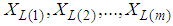 is given by
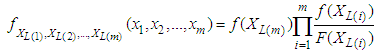 | (1) |
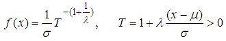 | (2) |
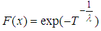 | (3) |
 is the shape parameter,
  is the scale parameter and
  is the location parameter.In this paper is organized in the following order: Section 2 provides Markov chain Monte Carlo’s algorithms. The maximum likelihood estimates of the parameters of the GEV distribution, the point and interval estimates of the parameters, as well as the approximate joint confidence region are studied in sections 3 and 4. The parametric bootstrap confidence intervals of parameters are discussed in section 5. Bayes estimation of the model parameters and Gibbs sampling algorithm are provided in section 6. Data analysis and Monte Carlo simulation results are presented in section 7. Section 8 concludes the paper.
2. MCMC Algorithms
- Markov chain Monte Carlo (MCMC) methods (which include random walk Monte Carlo methods) are a class of algorithms for sampling from probability distributions based on constructing a Markov chain that has the desired distribution as its equilibrium distribution. As computers became more widely available, the Metropolis algorithm was widely used by chemists and physicists, but it did not become widely known among statisticians until after 1990. Hastings (1970) generalized the Metropolis algorithm, and simulations following his scheme are said to use the Metropolis–Hastings algorithm. A special case of the Metropolis–Hastings algorithm was introduced by Geman and Geman (1984), apparently without knowledge of earlier work. Simulations following their scheme are said to use the Gibbs sampler. The state of the chain after a large number of steps is then used as a sample of the desired distribution. The quality of the sample improves as a function of the number of steps. MCMC techniques methodology provides a useful tool for realistic statistical modelling (Gilks et al. [14]; Gamerman, [15]), and has become very popular for Bayesian computation in complex statistical models. Bayesian analysis requires integration over possibly high-dimensional probability distributions to make inferences about model parameters or to make predictions. MCMC is essentially Monte Carlo integration using Markov chains. The integration draws samples from the required distribution, and then forms sample averages to approximate expectations (see Geman and Geman, [16]; Metropolis et al., [17]; Hastings, [18]).
2.1. Gibbs Sampler
- The Gibbs sampling algorithm is one of the simplest Markov chain Monte Carlo algorithms. The paper by Gelfand and Smith [19] helped to demonstrate the value of the Gibbs algorithm for a range of problems in Bayesian analysis. Gibbs sampling is a MCMC scheme where the transition kernel is formed by the full conditional distributions.
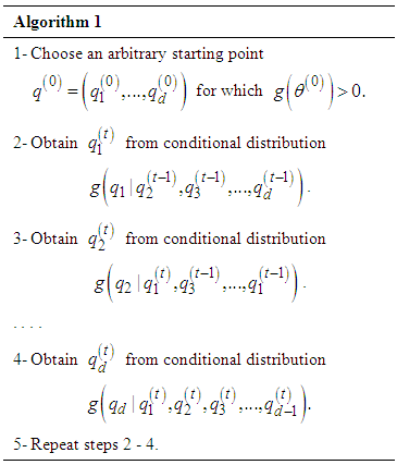 The Gibbs sampler is a conditional sampling technique in which the acceptance-rejection step is not needed. The Markov transition rules of the algorithm are built upon conditional distributions derived from the target distribution. The conditional posterior usually is but does not have to be one-dimensional.
2.2. The Metropolis-Hastings Algorithm
- The Metropolis algorithm was originally introduced by Metropolis et. al [17]. Suppose that our goal is to draw samples from some distributions
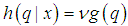 , where
  is the normalizing constant which may not be known or very difficult to compute. The Metropolis-Hastings (MH) algorithm provides a way of sampling from
  without requiring us to know
  . Let
. Let 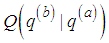 be an arbitrary transition kernel: that is the probability of moving, or jumping, from current state
  to
to . This is sometimes called the proposal distribution. The following algorithm will generate a sequence of the values
  , ... which form a Markov chain with stationary distribution given by
  .
.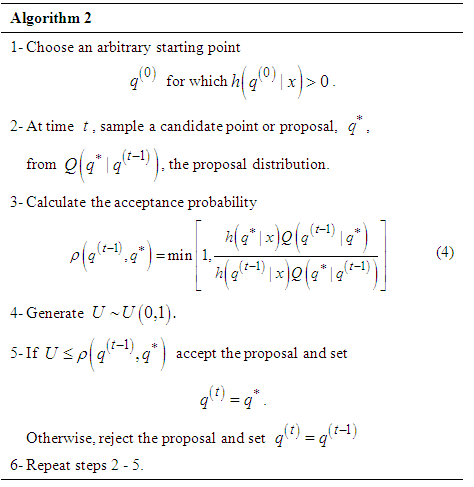 If the proposal distribution is symmetric, for all possible
  and
and  , so
, so  , in particular, we have
  , so that the acceptance probability (5) is given by:
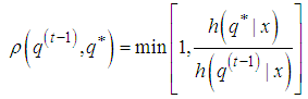 | (5) |
3. Maximum Likelihood Estimation
- Let
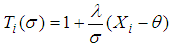
 be m lower record values each of which has the generalized extreme value whose the pdf and cdf are, respectively, given by (2) and (3). Based on those lower record values and for simplicity of notation, we will use
  instead of
  . The logarithm of the likelihood function may then be written as [20-23]:
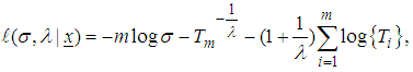 | (6) |
 with known
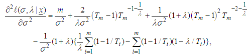
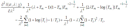
  . Calculating the first partial derivatives of Eq. (6) with respect to
  and
and  equating each to zero, we get the likelihood equations as:
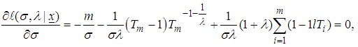 | (7) |
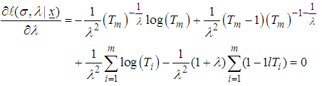 | (8) |
 and
and  say
say  and
and  .Records are rare in practice and sample sizes are often very small, therefore, intervals based on the asymptotic normality of MLEs do not perform well. So two confidence intervals based on the parametric bootstrap and MCMC methods are proposed.
4. Approximate Interval Estimation
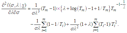
- If sample sizes are not small. The Fisher information matrix
 is then obtained by taking expectation of minus of the second derivatives of the logarithm likelihood function. Under some mild regularity conditions,
  is approximately bivariately normal with mean
  and covariance matrix
  . In practice, we usually estimate
  by
by  . A simpler and equally veiled procedure is to use the approximation
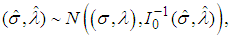 | (9) |
 is observed information matrix given by
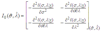 | (10) |
 | (11) |
 | (12) |
 | (13) |
 and
and  can be found by to be bivariately normal distributed with mean
  and covariance matrix
  Thus, the
  approximate confidence intervals for
  and
and  are:
are: | (14) |
 and
and  are the elements on the main diagonal of the covariance matrix
  and
and  is the percentile of the standard normal distribution with right-tail probability
  .
.5. Bootstrap Confidence Intervals
- In this section, we propose to use percentile bootstrap method based on the original idea of Efron [24]. The algorithm for estimating the confidence intervals of
 and
and  using this method are illustrated below.
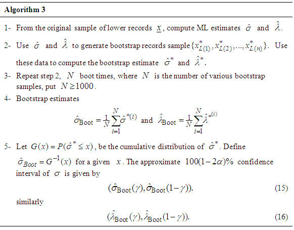
6. Bayesian Estimation
- In this section, we are in a position to consider the Bayesian estimation of the parameters
 and
and  for record data, under the assumption that the parameter
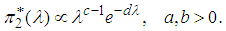
  is known. We may consider the joint prior density as a product of independent gamma distribution
  and
and  , given by
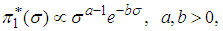 | (17) |
 | (18) |
 ,
,  and likelihood function, the joint posterior density function of
  and
and  given the data, denoted by
  can be written as
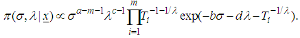 | (19) |
 given
given  is
is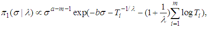 | (20) |
 given
given  can be written as
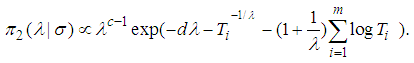 | (21) |
7. Data Analysis
- Now, we describe choosing the true values of parameters
 and
and  with known prior. For given
  generate random sample of size 100, from gamma distribution, then the mean of the random sample
 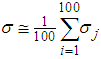 , can be computed and considered as the actual population value of
  That is, the prior parameters are selected to satisfy
  is approximately the mean of gamma distribution. Also for given values
  , generate according the last
  , from gamma distribution. The prior parameters are selected to satisfy
  is approximately the mean of gamma distribution. By using
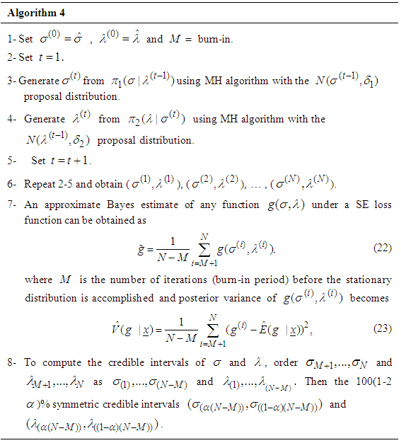
  , we generate lower record value data from generalized extreme lower bound distribution the simulate data set with
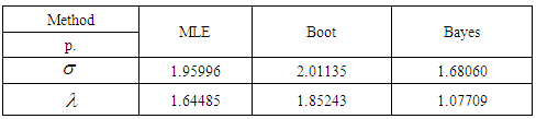
  , given by: 29.7646, 4.9186, 3.8447, 2.5929, 2.3330, 2.2460, 2.2348.Under this data we compute the approximate MLEs, bootstrap and Bayes estimates of
  and
and  using MCMC method, the MCMC samples of size 10000 with 1000 as 'burn-in'. The results of point estimation are displayed in Table 1 and results of interval estimation given in Table 2.
|
|
 of parameters σ and λ
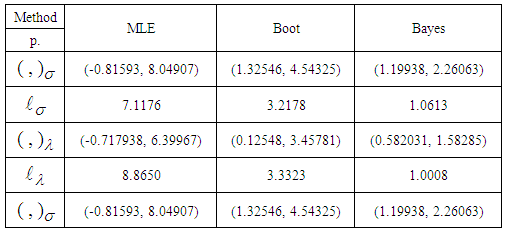
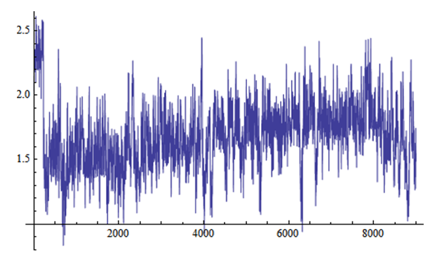 | Figure 1. Simulation number of σ generated by MCMC method |
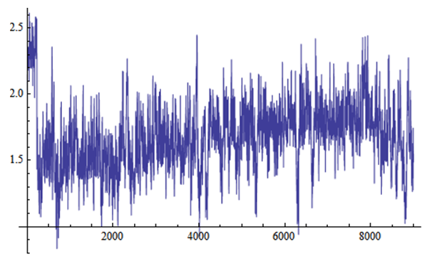 | Figure 2. Simulation number of λ generated by MCMC method |
8. Conclusions
- In the paper several algorithms of estimation of GEV distribution under the progressive Type II censored sampling plan are investigated. The asymptotic confidence intervals as well as bootstrap confidence are studied. The approximate confidence intervals, percentile bootstrap confidence intervals, as well as approximate joint confidence region for the parameters are expanded and developed. Some numerical examples with actual data set and simulated data are used to compare the proposed joint confidence intervals. The parts of MSEs and credible intervals lengths, the estimators of Bayes depend on non-informative implement more effective than the MLEs and bootstrap.
ACKNOWLEDGEMENTS
- The authors are grateful to anonymous referees who helped us to improve the presentation and their valuable suggestions, which improve the quality of the paper.