1. Introduction

A lot of variation can be seen from North to South and East to West of India. Top side of country is having a range of Mountains that starts from Jammu & Kashmir to Arunachal Pradesh; Middle part of country is having plains. Most of the south part of country is covered by sea. These parameters are responsible for the variation of climate that leads to cause of variations in rainfall that is why some parts of India are rich in rainfall and some parts of India are rain deficient.

In this blog, we have done analysis like forecasting of annual rainfall of Coastal Andhra for coming years. For the experiment, we have taken data of Mean Annual Rainfall from www.data.gov.in. The data is having the information of mean annual rainfall from year 1901 to 2016.

In this experiment we have taken the help of R programming that is now one of most demanded software in the field of data science and statistics. For the analysis, first column of the dataset is chosen to do analysis that is having annual mean rainfall information in mm unit.

2. Methodology

ARIMA models are capable of modelling a wide range of seasonal data. A seasonal ARIMA model is formed by including additional seasonal terms in the ARIMA models we have seen so far. It is written as follows:

ARIMA (p, d, q) (P, D, Q)m: the first parenthesis represents the non-seasonal part of the model and second represents the seasonal part of the model, where m= number of periods per season. We use uppercase notation for the seasonal parts of the model, and lowercase notation for the non-seasonal parts of the model. The additional seasonal terms are simply multiplied with the non-seasonal terms.

2.1. ACF/PACF

The seasonal part of an AR or MA model will be seen in the seasonal lags of the PACF and ACF. For example, an ARIMA(0,0,0)(0,0,1)12 model will show: a spike at lag 12 in the ACF but no other significant spikes. The PACF will show exponential decay in the seasonal lags; that is, at lags 12, 24, 36,….etc. Similarly, an ARIMA(0,0,0)(1,0,0)12 model will show: exponential decay in the seasonal lags of the ACF a single significant spike at lag 12 in the PACF. In considering the appropriate seasonal orders for an ARIMA model, restrict attention to the seasonal lags. The modelling procedure is almost the same as for non-seasonal data, except that we need to select seasonal AR and MA terms as well as the non-seasonal components of the model.

2.2. SARIMA

Seasonal autoregressive integrated moving average (SARIMA) model for any variable involves mainly four steps: Identification, Estimation, Diagnostic checking and Forecasting. The basic form of SARIMA model is denoted by and the model is given by 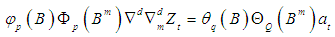where is the time series value at time t and are polynomials of order of p, P, q and Q respectively. B is the backward shift operator, and . Order of seasonality is represented by m. Non-seasonal and seasonal difference orders are denoted by d and D respectively. White noise process is denoted by . The Box-Jenkins methodology involves four steps (Box et al., 1994): (i) identification (ii) estimation (iii) diagnostic checking and (iv) forecasting. First, the original series must be transformed to become stationary around its mean and its variance. Second, the appropriate order of p and q must be specified using autocorrelation and partial autocorrelation functions. Third, the value of the parameters must be estimated using some non-linear optimization procedure that minimizes the sum of squares of the errors or some other appropriate loss function. Diagnostic checking of the model adequacy is required in the fourth step. This procedure is continued until an adequate model is obtained. Finally, the future forecasts generate using minimum mean square error method (Box et al. 1994). SARIMA models are used as benchmark models to compare the performance of the other models developed on the same data set. The iterative procedure of SARIMA model building was explained by Kumari et al. (2013), Boiroju (2012), Rao (2011) and Box et al. (1994).

2.3. ARIMA ( )

By default, the arima() command in R sets c=μ=0 when d>0 and provides an estimate of μ when d=0. The parameter μ is called the “intercept” in the R output. It will be close to the sample mean of the time series, but usually not identical to it as the sample mean is not the maximum likelihood estimate when p+q>0. The arima() command has an argument include.mean which only has an effect when d=0 and is TRUE by default. Setting include.mean=FALSE will force μ=0.

The Arima() command from the forecast package provides more flexibility on the inclusion of a constant. It has an argument include.mean which has identical functionality to the corresponding argument for arima(). It also has an argument include.drift which allows μ≠0μ≠0 when d=1. For d > 1, no constant is allowed as a quadratic or higher order trend is particularly dangerous when forecasting. The parameter μμ is called the “drift” in the R output when d=1.

This is also an argument include.constant which, if TRUE will see include.mean=TRUE if d=0 and include.drift=TRUE when d=1. If include.constant=FALSE. Both include.mean and include.drift will be set to FALSE. If include.constant is used, the values of include.mean=TRUE and include.drift=TRUE are ignored.

2.4. auto.arima ( )

The auto.arima() function automates the inclusion of a constant. By default, for d=0 or d=1, a constant will be included if it improves the AIC value; for d > 1, the constant is always omitted. If allow drift=FALSE is specified, then the constant is only allowed when d=0.

There is another function arima() in R which also fits an ARIMA model. However, it does not allow for the constant cc unless d=0, and it does not return everything required for the forecast() function. Finally, it does not allow the estimated model to be applied to new data (which is useful for checking forecast accuracy). Consequently, it is recommended that you use Arima() instead.

2.5. Modelling Procedure

When fitting an ARIMA model to a set of time series data, the following procedure provides a useful general approach.

1. Plot the data. Identify any unusual observations.

2. If necessary, transform the data (using a Box-Cox transformation) to stabilize the variance.

3. If the data are non-stationary: take first differences of the data until the data are stationary.

4. Examine the ACF/PACF: Is an AR(pp) or MA(qq) model appropriate?

5. Try your chosen model(s), and use the AICc to search for a better model.

6. Check the residuals from your chosen model by plotting the ACF of the residuals, and doing a portmanteau test of the residuals. If they do not look like white noise, try a modified model.

7. Once the residuals look like white noise, calculate forecasts.

2.6. AIC and BIC

AIC and BIC are both penalized-likelihood criteria. They are sometimes used for choosing best predictor subsets in regression and often used for comparing non-nested models, which ordinary statistical tests cannot do. The AIC or BIC for a model is usually written in the form [-2logL + kp], where L is the likelihood function, p is the number of parameters in the model, and k is 2 for AIC and log(n) for BIC.

AIC is an estimate of a constant plus the relative distance between the unknown true likelihood function of the data and the fitted likelihood function of the model, so that a lower AIC means a model is considered to be closer to the truth. BIC is an estimate of a function of the posterior probability of a model being true, under a certain Bayesian setup, so that a lower BIC means that a model is considered to be more likely to be the true model. Both criteria are based on various assumptions and asymptotic approximations. Each, despite its heuristic usefulness, has therefore been criticized as having questionable validity for real world data. But despite various subtle theoretical differences, their only difference in practice is the size of the penalty; BIC penalizes model complexity more heavily. The only way they should disagree is when AIC chooses a larger model than BIC.

AIC and BIC are both approximately correct according to a different goal and a different set of asymptotic assumptions. Both sets of assumptions have been criticized as unrealistic. Understanding the difference in their practical behaviour is easiest if we consider the simple case of comparing two nested models. In such a case, several authors have pointed out that IC’s become equivalent to likelihood ratio tests with different alpha levels. Checking a chi-squared table, we see that AIC becomes like a significance test at alpha=0.16, and BIC becomes like a significance test with alpha depending on sample size, e.g., 0.13 for n = 10, .032 for n = 100, .0086 for n = 1000, .0024 for n = 10000. Remember that power for any given alpha is increasing in n. Thus, AIC always has a chance of choosing too big a model, regardless of n. BIC has very little chance of choosing too big a model if n is sufficient, but it has a larger chance than AIC, for any given n, of choosing too small a model.

In general, it might be best to use AIC and BIC together in model selection. For example, in selecting the number of latent classes in a model, if BIC points to a three-class model and AIC points to a five-class model, it makes sense to select from models with 3, 4 and 5 latent classes. AIC is better in situations when a false negative finding would be considered more misleading than a false positive, and BIC is better in situations where a false positive is as misleading as, or more misleading than, a false negative.

3. Forecasting of Rainfall of Coastal Andhra

The data has been taken to predict the rain fall of coastal area of Andhra Pradesh from the year 1951 to 2016. The data has monthly rainfall for each year. In this section, we have to check forecasting model to this data using one of statistical tool R software. In R software majorly we need packages for forecasting model. Using these packages is predicting the model for the coastal data. The packages are ‘ggplot2’, ‘forecast’ and ‘tseries’. Install the above mentioned packages using install.packages() function and call that packages using library function as below:

Library ('ggplot2') # calls the packages using Library ().

Library ('forecast')

Library ('tseries')

The data has been converted into “.csv” file and then read the data into the R programming.

CA<-read.csv ("D:/ganesh/statistics Softwares/project/Analysis2017/Ganesh/CA.csv") # to read the data

To find the summery of the rainfall of coastal Andhra, the following command can be use:

Summary (CA) # to see basic details of data set.

Summery details:

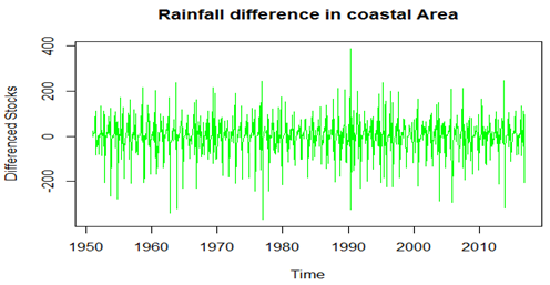
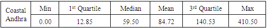The minimum and maximum rainfall is 0.00 and 410.50, first and third quartiles are 12.85 and 140.53. Basing on the quartile, the deviation is 63.84. Average rainfall of coastal is 84.42 and median rainfall is 59.50. Depending on the above summery, we cannot give any decision about the rainfall of coastal Andhra.

To know the pattern of the data, we have applied the below mentioned time series command.

Myts <- ts (CA [, 3], start=c (1951, 1), end = c (2016, 12), frequency = 12) # Applying time series to data.

If you draw the graph of the rainfall, we can observe whether the data is in stationary or not. To check the stationary of the data we have applied Augmented Dickey-Fuller test. The test is significant (p<0.05*), so that the data is stationary and we can observe in the graph of the data and its difference.

Plot (Myts, xlab='year', ylab = 'Stocks', main="Rainfall difference in coastal Area", col="blue") # Graph for time series data.

adf.test (myts, alternative = "stationary") # Stationary checking

Augmented Dickey-Fuller Test

Dickey-Fuller = -12.829, Lag order = 9, p-value = 0.01

Alternative hypothesis: stationary

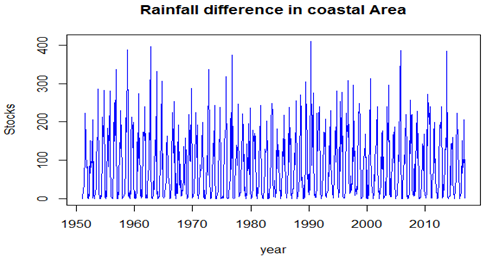Dec <- decompose (Myts) # using decompose function to see the decompose details.

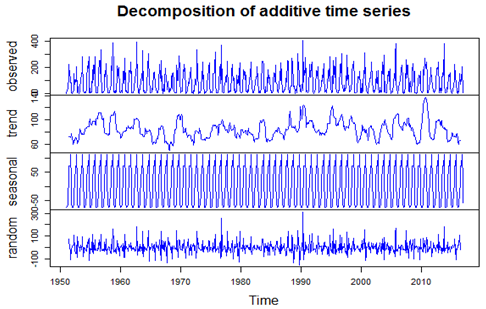The above four graphs represents the original data, seasonal component, trend component and the remainder and this shows the periodic seasonal pattern extracted out from the original data and the trend. There is a bar at the right hand side of each graph to allow a relative comparison of the magnitudes of each component. For this data the change in trend is less than the variation doing to the monthly variation.

ARIMA model for data: we are using auto arima method for find forecasting model for data set.

ARIMAfit <- auto.arima (Myts, approximation=FALSE, trace=FALSE) # to build forecasting model

To check the details of ACF and PCF of Rain fall data.

Acf (ts (Myts), main='ACF Tractor Sales’, col="blue")

Pacf (ts (Myts), main='PACF Tractor Sales’, col="green")

The entire document should be in Times New Roman. The font sizes to be used are specified in Table 1.

The size of a lower-case “j” will give the point size by measuring the distance from the top of an ascender to the bottom of a descender.

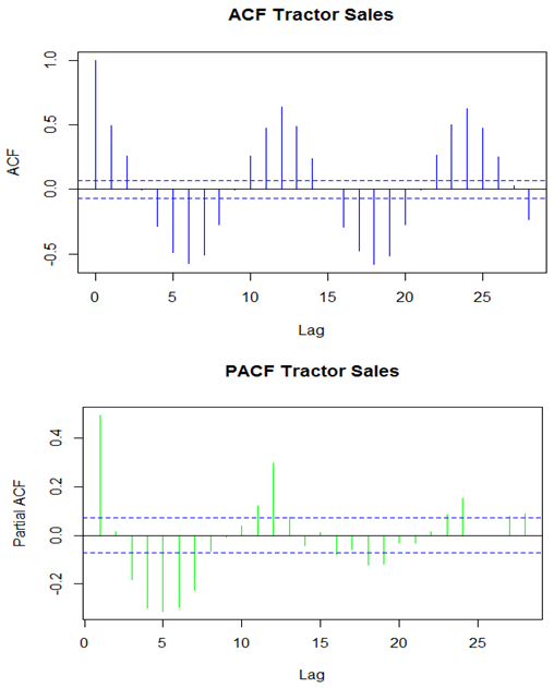The ACF plot of the residuals from the ARIMA (1,0,0)(2,0,0)[12] model shows all correlations within the threshold limits indicating that the residuals are behaving like white noise. A portmanteau test returns a large p-value, also suggesting the residuals are white noise. The PACF shown is suggestive of model. So an initial candidate model is an ARIMA (1,0,0)(2,0,0)[12]. There are no other obvious candidate models.

3.1. ARIMA (1,0,0)(2,0,0)[12] with Non-zero Mean

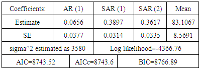Automate ARIMA model for the data is ARIMA (1,0,0)(2,0,0)[12] with non-zero mean. The predicted values for coast area rain fall details using ARIMA method of (1, 0, 0) and (2, 0, 0).

By applying auto ARIMA, we got the best fitted model which has the lowest AICc. When models are compared using AICc values, it is important that all models have the same orders of differencing. However, when comparing models using a test set, it does not matter how the forecasts were produced - the comparisons are always valid. The given model has been passed the residual tests. In practice, we would normally use the best model we could find, even if it did not pass all tests. Forecasts from the ARIMA(1,0,0)(2,0,0)[12] model are shown in the figure below.

Fact <- forecast (ARIMAfit, h=60) #forecasting values

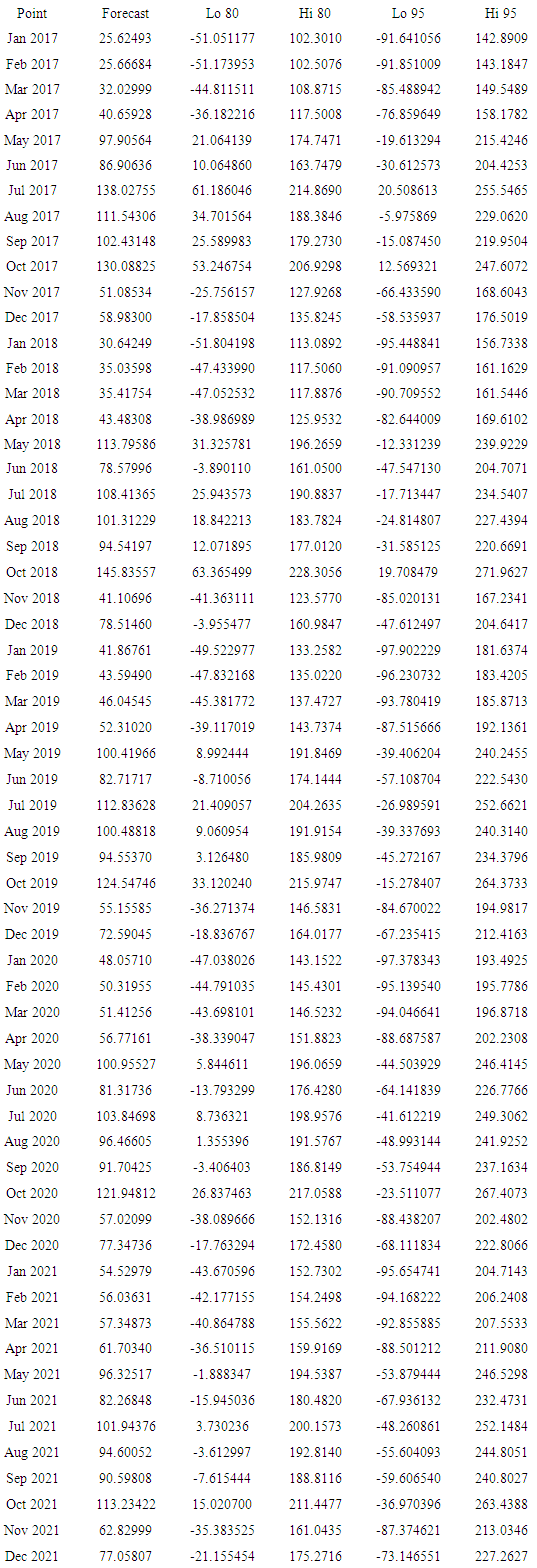plot(fact) # Plot the actual and forecast values

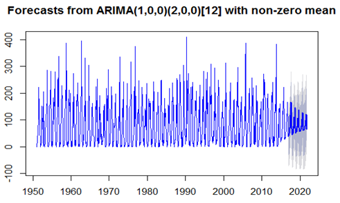
3.2. Forecasting for Seasonal Differences

In this section, we have considered the rainfall data with differences. The same interpretation has been carried out for the below mentioned model.

Plot (diff (Myts), main="Rainfall difference in coastal Area", ylab='Differenced Stocks', col="green") Graph for time series difference data

To check the details of ACF and PCF of Rain fall data differences.

Acf (ts (diff (Myts)), main='ACF Tractor Sales’, col="blue")

Pacf (ts (diff (Myts)), main='PACF Tractor Sales’, col="green")

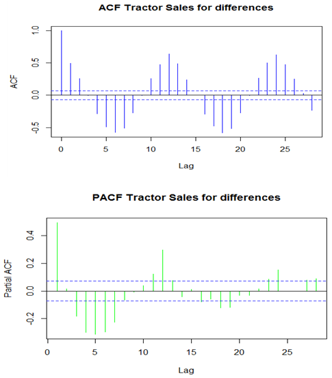ARIMAfit <- auto.arima (diff (Myts), approximation=FALSE, trace=FALSE) # difference in data.

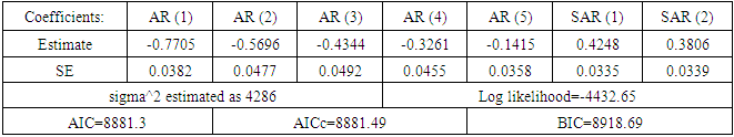
3.3. ARIMA (5,0,0)(2,0,0)[12] with Zero Mean

Fact<- forecast (ARIMAfit, h=60)

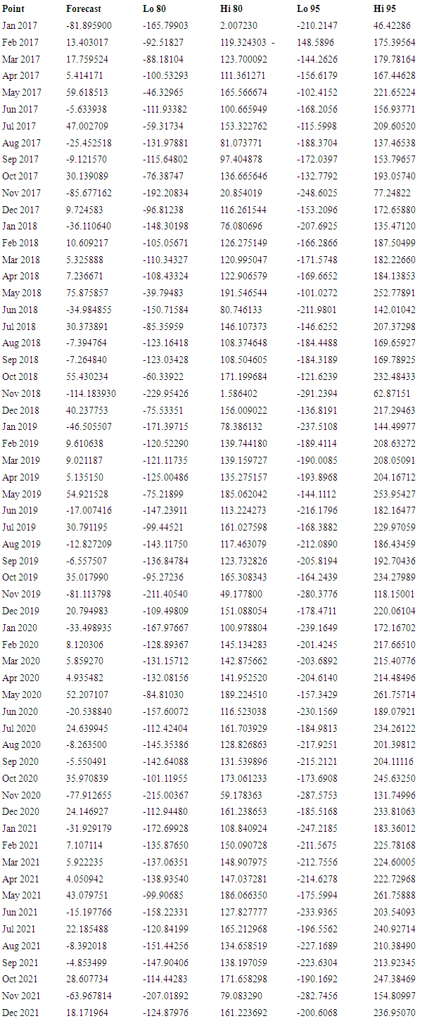Plot (fact)

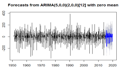
4. Conclusions

The data has been fitted to the ARIMA (5, 0, 0) (2, 0, 0)[12] model for rainfall of coastal Andhra. Augmented Dickey-Fuller Test has been tested for stationarity of the data. Basing on the p-value (p=0.01), the data has been stationary and we have applied for auto ARIMA to find and check the best model using R. We have made the interpretation basing on the AIC and BIC values of the model. The lowest AIC and BIC will give us the best fit of the forecast model. Based on auto ARIMA, the best fitted model has been found ARIMA (5, 0, 0) (2, 0, 0)[12], which has the seasonality. The prediction values and its graphs have been shown.

ACKNOWLEDGEMENTS

The authors thank the referees for their valuable comments which have improved the presentation of the paper.