Shei Sayibu Baba1, Tuahiru Maahi2
1Department of Statistics, Faculty of Mathematical Sciences, University for Development Studies, Navrongo, Ghana
2Department of Statistics and Mathematics, School of Applied Science and Technology, Tamale Technical University, Ghana
Correspondence to: Shei Sayibu Baba, Department of Statistics, Faculty of Mathematical Sciences, University for Development Studies, Navrongo, Ghana.
| Email: |  |
Copyright © 2017 Scientific & Academic Publishing. All Rights Reserved.
This work is licensed under the Creative Commons Attribution International License (CC BY).
http://creativecommons.org/licenses/by/4.0/

Abstract
In this study, we propose a unified Cumulative Sum (CUSUM) control chart for monitoring simultaneous shifts in the parameters of the Pareto distribution. The V-mask method of constructing a CUSUM control chart was used. The characteristics of the V-mask were investigated and it was observed that the lead distance, the mask angle and the Average Run Length (ARL) of the CUSUM control chart changed considerably for a small shift in the parameters of the Pareto distribution.
Keywords:
Unified CUSUM, Run length, Lead distance, V-Mask and simultaneous
Cite this paper: Shei Sayibu Baba, Tuahiru Maahi, Unified Cumulative Sum Control Chart for Moniroring Shifts in the Parameters of the Pareto Distribution, International Journal of Statistics and Applications, Vol. 7 No. 3, 2017, pp. 170-177. doi: 10.5923/j.statistics.20170703.02.
1. Introduction
The quality of a product cannot be underestimated by both producers and consumers. Industry players therefore need a robust procedure to meet this desired quality and one of such procedures include the CUSUM control chart. The CUSUM control chart was proposed first by Page (1954) as a built up of the work done by Shewhart (1926). The Shewhart control charts are not able to detect a small to medium size shift in the process parameter. The CUSUM control chart has the tendency to detect this small to moderate size shift in the process parameter. Many researchers have studied enormously into the arena of CUSUM control charts. Notably among them include: Hawkins and Olwell (1998) stated that the CUSUM control charts are most sensitive Statistical Process Contol (SPC) to signal a persistent small step change in a process parameter. Also, Luguterah (2015) developed unified CUSUM control chart for monitoring simultaneous shifts in the parameters of the Elang-Truncated Exponential Distribution and therefore derived the parameters of the CUSUM chart proposed. Again, Naber and Bilgi (1994) developed a CUSUM control chart for the Gaussian distribution. Again, Kantam and Rao (2004) investigated the CUSUM control chart for the Log-Logistic Distribution and concluded that it was able to detect shifts on the average than the Shewhart control charts. Sasikumar and Bangusha (2014) explained the common uses of CUSUM control charts for monitoring performance overtime when the outcome is related to health science. The article provided a logical way to accumulate evidence over many patients, while adjusting for a changing mix of patients’ characteristics that significantly affected risk. Bakhodir (2004) employed CUSUM control chart in economic and finance turning point in stock price indices.Recently, Nasiru (2016) developed a one-sided CUSUM control chart for monitoring the shape parameter of the Pareto distribution.In this study, we extended the study of Nasiru (2016) and therefore develop a two-sided CUSUM control chart for monitoring shifts in the shape parameter of the Pareto distribution.
2. Pareto Distribution
The Pareto distribution is lop-sided and a heavy-tailed distribution which was developed by the Italian economist and sociologist, Vilfredo Pareto (1848 – 1923). He worked in the field of national economy and sociology. The Pareto distribution is applied in modeling problems involving distributions of incomes or wealth and also many situations in which there will always be a shift in the equilibrium of the system.If the random variable X has a Pareto distribution, then the density function is given by;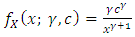 | (1) |
where  and the parameters
  and
and  are the shape and scale parameters respectively. The corresponding cumulative distribution function is given by;
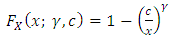 | (2) |
The mean and variance of the Pareto distribution are given by;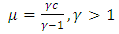 | (3) |
and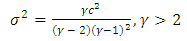 | (4) |
respectively.
3. Sequential Probability Ratio Test
The Sequential Probability Ratio Test (SPRT) plays a significant role in the development of an acceptance sampling plan. The Wald’s (1947) SPRT is a joint, subject by subject, Likelihood Ratio Test (LRT). In this approach each subject constitutes a stage. According to Johnson (1961), the CUSUM control charts are roughly equivalent to the SPRT. The SPRT have been used extensively in the development of an acceptance sampling plan and this acceptance sampling plan is used in determining the in and out-of-control limits in CUSUM procedures.Suppose that we take a sample of m values  successively, from a population
  . Consider two hypotheses about
  ,
,  and
and  . The ratio of the probabilities of the sample is;
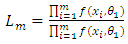 | (5) |
We select two numbers A and B, which are related to the desired  and
and  errors. The sequential test is set up as follows;i. As long as
  we continue sampling.ii. At the first i that
  we accept
  .iii. At the first i that
  we accept
  .An equivalent way for computation is to use the logarithm of
  . Then, the inequality becomes;
 | (6) |
The family of test is referred to as SPRT. If 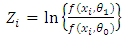 | (7) |
then the sampling terminates when | (8) |
or  | (9) |
The  are independent random variables with variance, say,
  . Obviously
  has a variance
  . As
. As  increases the dispersion becomes greater and the probability that a value of
  will remain within the limits
  and
and  tends to zero. The mean
  tends to a normal distribution with variance
  and therefore the probability that it will fall between
  and
and  tends to zero.If we take a sample for which
  lies between A and B for the first
  trial and then
  at the
  trial, so we accept
  (and reject
  ). By definition, the probability of getting such a sample is at least A times as large under
  as against
  . The probability that we fail to reject
  when
when  is true is
  and the probability that we reject
  when
when  is true is
  . Therefore
 | (10) |
Similarly, if we accept 
 | (11) |
Wald (1947) showed that for all practical purposes (10) and (11) holds as equalities. Thus | (12) |
and | (13) |
Suppose that  and
and  and that the true errors of first and second kind for the limits
  and
and  are
are  and
and  respectively. Then, from (10)
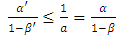 | (14) |
and from (11)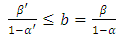 | (15) |
Therefore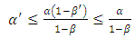 | (16) |
and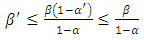 | (17) |
Furthermore | (18) |
In practice  and
and  are small. From (16) and (17), the amount that
  can exceed
  or
or  exceed
  is negligible. In addition, from relation (18) we see that either
  or
or  . Therefore the use of
  and
and  can only increase one of the errors and only by a very small amount
4. CUSUM Control Chart for Monitoring the Shape (γ) and Scale Parameters (c)
In this section a unified CUSUM chart for monitoring both the scale and shape parameters of the Pareto distribution was constructed. The likelihood ratio test of the null hypothesis which says that there is no shift in the parameters of the Pareto distribution against the alternative that there is a shift in the parameters of the Pareto distribution is given as follows: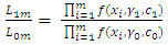 | (19) |
 | (20) |
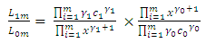
The continuation region of the SPRT that discriminates between the two hypotheses is given by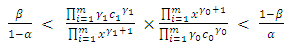 | (21) |
which becomes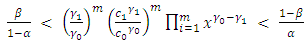 | (22) |
taking natural logarithm of both sides of (23) | (23) |
Bearing in mind that the mean and variance of the Pareto distribution, any shift in the parameters affects these two moments. Let  and
and  be the target values, let also
  and
and  be the changed values owing to the shift in the parameters. The SPRT will be stopped by rejecting or accepting the null hypothesis or continue to sample, as
  is outside or between
  and
and  . The process stops by rejecting
  if
if  ; this gives a rejection line
  and
and  . Similarly, if we make use of SPRT with the same strength to the cases
  and
and  , where
 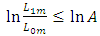 , then another rejection line is determined. These two rejection lines indicates a symmetrical nature of masking. The observations in the sample enter the mask in a sequential way. Thus, the mask for the CUSUM chart for
  is
is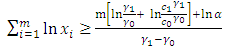 | (24) |
This implies 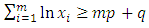 | (25) |
where and
and Similarly, the rejection line, when
  , is given by
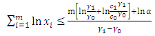 | (26) |
which can be expressed as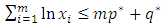 | (27) |
where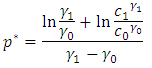 and
and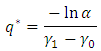 Equations (26) and (28) form the regions above and below the plane
  . If m is allowed sequentially, at some stage,
  satisfies either (26) or (28). Until this is achieved the process continues.Using the slopes of the two lines (equations (26) and (28)), the parameters of the CUSUM chart, known as the angle of the mask and the lead distance, are obtained. From Figure 1,
  slope of the line
  and
and  slope of the line
  , hence
 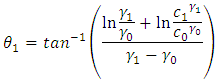 where
where  and
and  .And
.And 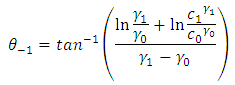 where
where  and
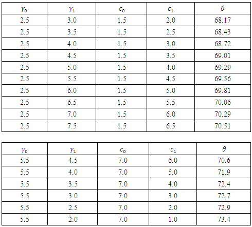
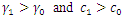
and  .Various values of the angle are shown in Table 1. It was obvious from the results that as the values of
  and
and  increase the value of the angle increases. Also increasing values of
  and
and  also increase the angle of the mask.
 Table 1. Values of the angle θ for controlling both γ and c
 |
| |
|
When there is a negative shift in both parameters, that is where  and
and  , it can be established from the second table of Table 1 that the mask angle
  increases as the values of
  and
and  decreases.The lead distance
  is given by
  where
where  and
and  and the lead distance
  is given by
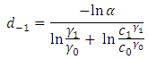 where
where  and
and  .Let
.Let  be a sample from Pareto distribution, if the points
 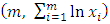 are plotted with a suitable scale, then the ordinates of the points represent the cumulative sum of the data. Equations (26) and (28) are the effects of a shift in the population parameters
  and
and  . Figure 1 shows a sizable shift in the parameters if
  falls outside the lines
  and
and  . The chart is interpreted by placing the mask over the last plotted point as shown in Figure 1. If any of the points lies below
  , then it indicates a decrease in
  and
and  and if any of the points falls above
  , then it shows an increase in
  and
and  .
.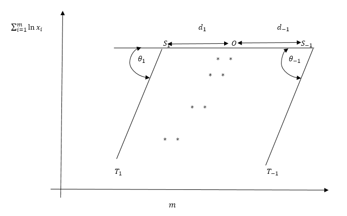 | Figure 1. V-mask for unified CUSUM control chart |
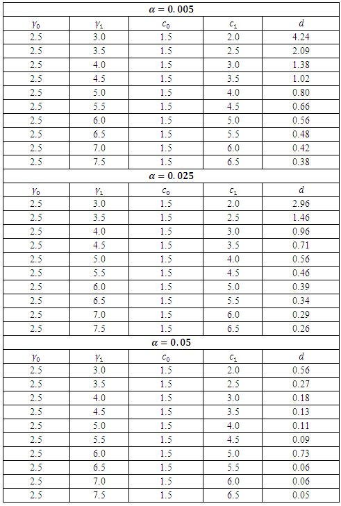
Using some hypothetical values for  and
and  , it can be determined that increasing the values of
  and
and  , the lead distance decreases given a fixed value of
  . Again, the value of also increases with decreasing values of
  and a given fixed value of
  and
and  . The details of the values of the lead distance are shown in Table 2.
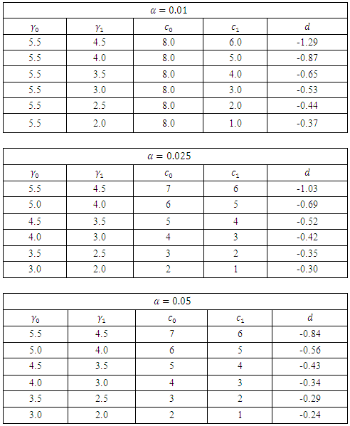
Table 2. Values the lead distance d for controlling γ and c when
 |
| |
|
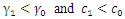
On the other hand, when there is a negative shift of the parameters, that is  and
and  , it can be established that the lead distance (d) decreases as the value of alpha
  increases and when the value of
  and
and  decreases for a fixed value of
  , the value of the lead distance increases. The details are shown in Table 3. The values of the lead distance are negative in this case because there is a negative shift in the parameters of the distribution.
Table 3. Values the lead distance d for controlling γ and c when
 |
| |
|
5. Average Run Length of the Unified CUSUM Control Chart
The Average Run Length of the unified CUSUM chart is the same as that of the two-sided CUSUM chart and is given by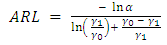 | (28) |
Proof:By definition 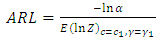 | (29) |
where 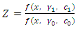 .using equation (1),
  can be written as
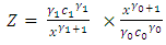 | (30) |
Taking natural logarithm of (30)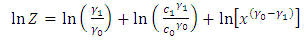 | (31) |
By simplifying (31), it reduces to 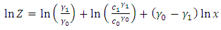 | (32) |
Taking expectation of (32)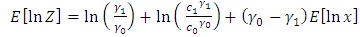 | (33) |
The expectation,  is obtained as follows
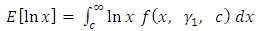 | (34) |
By substituting the density function for  into (34), we obtained
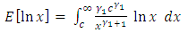 | (35) |
Simplifying (35), we obtained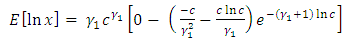 | (36) |
and finally, | (37) |
Substituting the value of  in (37) into (33) we obtain
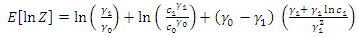 | (38) |
Simplifying (38), we obtain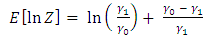 | (39) |
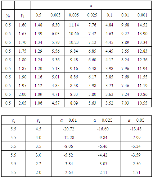
Substituting (39) into (29), the ARL formular is derived as required.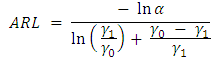 Using some hypothetical values of
  and
and  , it can be established that as
  increases in value, the ARL tends to decrease with any given value of
  . Also as the value of
  decreases, the ARL also increases for fixed value of
  as displayed in Table 4.
 Table 4. Average Run Length for the parameters of the Pareto distribution
 |
| |
|
Also it can be established in the second table of Table 4 that when there is a negative shift  , the ARL decreases as
  increases and when
  decreases, the ARL also increases for any given value of
  . The negative values of the ARL obtained only indicates the negative shift in both parameters of the Pareto distribution.
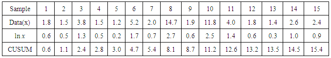
6. Practical Demonstration of the Unified CUSUM Control Chart
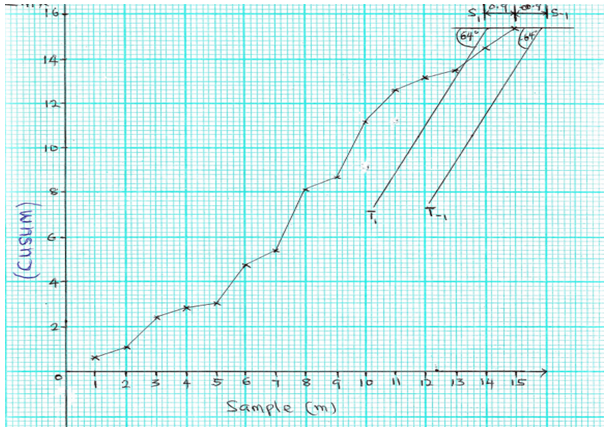
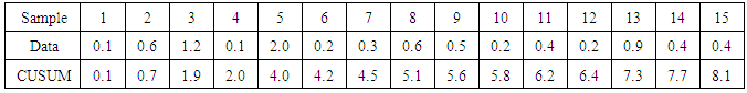
In this section, the application of the proposed CUSUM chart has been illustrated using a hypothetical data simulated from the Pareto distribution. The first ten observations were simulated with  and
and  . The last five observations were simulated with
  and
and  for a simultaneous shift in both parameters. Table 5 displays the simulated data points and the corresponding cumulative sum. The parameters of the V-mask were calculated using
  ,
,  ,
,  ,
,  and
and  . The lead distance and the mask angle were obtained as 0.9 and
  respectively. The sample number
  was plotted against the cumulative sum of the data. The V-mask was then placed at the last plotted point to monitor whether the process is in control or out of control as shown in Figure 2. It can be established from Figure 2, the process was out of control as observations 1 to 13 fell above line
  indicating an increase in
  and
and  . On the other hand if the plotted points fall below the line
  , means there is a negative shift in the parameters. Anytime any of the above scenarios are experience then an action should be taken in order to bring the process back to control.
Table 5. Simulated hypothetical data for the unified CUSUM
 |
| |
|
 | Figure 2. Unified CUSUM plot for the simulated hypothetical data |
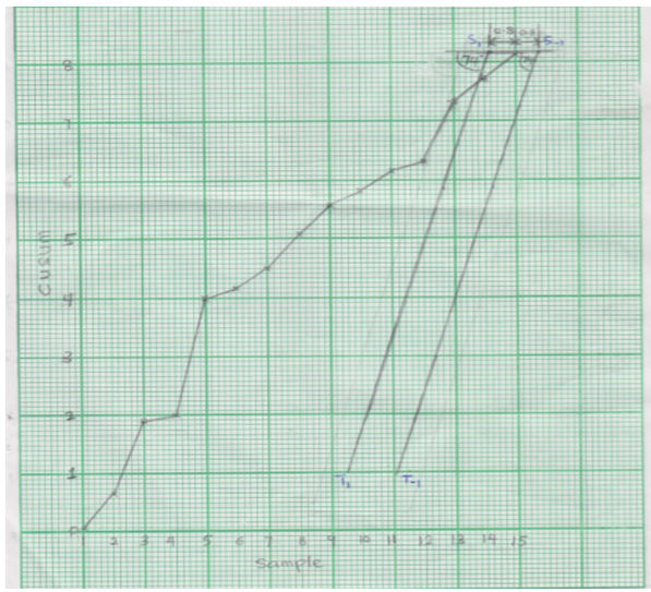
In Table 6, the first ten observations were simulated with  and
and  . The last five observations were simulated with
  and
and  for a simultaneous shift in both parameters. The parameters of the V-mask were calculated using
  ,
,  ,
,  ,
,  and
and  . The lead distance and the mask angle were obtained as - 0.8 and
  respectively. Since distance cannot be negative, an absolute value of the distance was then used in the placing of the V-mask. The sample number was then plotted against the cumulative sum (CUSUM) of the data. The V-mask was then placed at the last plotted point to monitor whether the process is in control or out of control as shown in Figure 3. It was established from Figure 3 that the process was out of control as observations 1 to 13 fell above line
  indicating a shift in
  and
and  . This calls for a corrective measure to be taken in order to bring the process back to control.
Table 6. Simulated hypothetical data for the unified CUSUM
 |
| |
|
 | Figure 3. Unified CUSUM plot for the simulated hypothetical data |
7. Conclusions
The results of the study showed that as the values of  and
and  increase the size of the mask angle
  increases. Also, increasing values of
  and
and  increases the size of the mask angle
  . Furthermore, when there is a negative shift in both parameters, that is where
  and
and  , it can be established from the second table of Table 1 that the mask angle
  increases as the values of
  and
and  decreases.With regard to the lead distance it can be determined that increasing the values of
  and
and  , the lead distance decreases given a fixed value of
  . Again, the value of the lead distance increases with decreasing values of
  and a fixed value of
  and
and  . However, When there is a negative shift in the parameters of the distribution, that is
  and
and  , it can be established that the lead distance decreases as the value of alpha
  increases and when the value of
  and
and  decreases for a fixed value of
  , the value of lead distance increases. On the ARL, it was established that as
  increases in value, the ARL tends to decrease with any given value of
  . Also, as the value of
  decreases, the ARL also increases for a fixed value of
  . Again when there is a negative shift
  , the ARL decreases as
  increases and when
  decreases, the ARL also increases for any given value of
  .
.
References
| [1] | Bakhodir, E. A. (2004). Sequential Detection of U.S. Business Cycle Turning points: performances of Shiryayev-Roberts, CUSUM and EWMA procedures. Econ, papers, submitted for publication. |
| [2] | Hawkins, D. M. and Olwell D. H. (1998). Cumulative sum charts and charting for quality improvement. Springer-Verlag, New York. |
| [3] | Johnson, N. L. (1961). A simple theoretical approach to cumulative sum control charts. Journal of the American Statistics Association, 56(4): 835-40. |
| [4] | Kantam, R. R. L. and Rao, G. S. (2004). A note on point estimation of system reliability exemplified for the Log-logistic distribution. Economic Quality control. 19(2): 197-204. |
| [5] | Luguterah, A. (2015). Unified cumulative sum chart for monitoring shifts in the parameters of the Erlang-Truncated exponential distribution. Far East Journal of Theoretical Statistics, 50(1): 65-76. |
| [6] | Nabar, S. P. and Bilgi, S. (1994). Cumulative Sum Control chart for the Inverse Gaussian distribution. Journal of Indian Statistical Association. 32:9-14. |
| [7] | Nasiru, S. (2016). One-sided cumulative sum control chart for monitoring shifts in the shape parameter of Pareto distribution. Int. J. Productivity and Quality Management, 19(2): 160. |
| [8] | Page E. S. (1954). Continuous Inspection Schemes. Biometrics, 41(1): 100-115. |
| [9] | Sasikumar, R. and Bangusha, D. S. (2014). Cumulative sum charts and its Health care Applications - A systematic Review. SriLangan Journal of Applied Statistics. 15(1):47-56. |
| [10] | Shewhart, W. A. (1926). Quality Control Charts. Bell Syst. Tech. J. 5:593-602. |
| [11] | Wald, A. (1947). Sequential Analysis. |

 Abstract
 Reference
 Full-Text PDF
 Full-text HTML