1. Introduction

Extreme market risk is an important type of financial risk, which is generally caused by extreme price movements in the financial market. Although this risk occurs in small probabilities, it can cause disastrous consequences on the market by engendering substantial financial losses. Glaring evidences of it are serious financial disasters that have occurred in the past, such as the notorious market crash commonly known as the ‘Black Monday’ which took place in the US in October 1987, also the 1997-1998 Asian crisis and the subprime crisis of 2007-2009. This random risk has prompted researchers, regulators and policymakers to develop diverse methodologies to understand the likelihood and extent of extreme rare events which help explain stock market crashes or currency crises, losses on financial assets, catastrophic insurance claims, credit losses or even losses incurred due to natural disasters.

Value-at-Risk (VaR) is a popular tail-related risk measure which provides a reasonable and realistic quantification of extreme market risk.

It is extensively used by investors, banks, traders, financial managers and regulators to monitor the level of risk.

According to to Jorion [1], Value-at-Risk (VaR) is the worst loss that will not be exceeded with a certain level of confidence, during a particular period of time. It is often associated with extreme downside losses caused by extreme deviations in market conditions. So much so, that the necessity to accurately estimate VaR has led to the development of diverse methodologies for extreme risk management.

The Generalised Autoregressive Conditional Heteroskedasticity (GARCH) model by Bollerslev [2] was developed as an extension to the Autoregressive Conditional Heteroskedasticity (ARCH) by Engle [3]. GARCH are robust techniques developed for the modelling of high frequency time series data. Past experiments show that they efficiently capture the stylised feature of volatility clustering in financial data. GARCH models are therefore most often used to forecast volatility and subsequently Value-at-Risk (VaR), [4]. According to [5] and [6], the GARCH(1,1) specification is the most widely used and has proved to be a successful volatility technique in many past studies. Nevertheless, other mathematical explanations have been proposed to enlighten the issue of fat tails in modeling extreme market risk. For instance, Blattberg & Gonedes [7] and Bollerslev [2] contributed to the implementation of t distribution, to account for fat-tailed return distributions. Similarly, other several studies have attempted to challenge the general Gaussian assumption and provide better techniques to model tail-risk measure VaR, such as the Extreme Value Theory (EVT).

Extreme Value Theory (EVT) is a robust tool for studying the tail of a distribution as it provides a plausible theoretical foundation whereby statistical models, which describe extreme and rare events, can be constructed. The roots of EVT began with the early pioneering work of Frechet (1927), Fisher & Tippett (1928), Gnedenko (1943) and Gumbel (1958). Balkema and de-Haan (1974) as well as Pickands (1975) further explored the theory and presented important results for threshold-based extreme value techniques. Since then, EVT has proved to be useful in many spheres of life, including Finance. EVT is basically a parametric model which captures the extreme tails of a distribution in order to forecast risk. It allows the estimation of extreme quantiles, making it an attractive model for Value-at-Risk (VaR) estimation, as it provides better distributions to fit those extreme data. There are two main modelling methods for EVT namely the Block Maxima Method (BMM) and the Peak Over Threshold (POT) method. The POT is often preferred over BMM as the former approach makes efficient use of the available data by picking all relevant observations beyond a particular high threshold while the latter approach considers only the extreme values in specified blocks. In addition, POT model has the advantage that it does not require a large data set as the BMM model, [8, 9].

In 1975, Pickands devised the theoretical framework and statistical tools for the POT method whereby only those observations which exceed a particular sufficiently high threshold are considered. Under extreme value conditions, the absolute exceedances over the threshold value u are said to follow the Generalised Pareto Distribution (GPD) as per the Pickands, Balkema-in Haan Theorem. Past studies have shown that compared to the BMM approach, it is easier to compute VaR based on the POT approach [10].

Many studies based on the performance on VaR-EVT models have been conducted in the past. Gencay & Selcuk [11] have examined the relative performance of VaR models in nine different emerging markets. They found that EVT-based VaR estimates were the most accurate at higher quantiles. Moreover, Danielsson & Morimoto [12] studied the forecasting performance of EVT-based VaR model in the Japanese economy where traditional GARCH-type methods were compared to EVT. They found that distribution of extremes, clustering, asymmetry, as well as the dynamic structure of VaR are important criteria to be considered during comparison of the various methods. They also concluded that the inaccuracy and the high volatility of the VaR forecasts made GARCH models unsuitable while EVT gave better and more stable VaR estimates. Several other researchers have attempted to analyse extreme fluctuations in financial markets. Most of them have provided details on the tail behaviour of financial data and examined the prospect of EVT as a risk management tool [8, 13-17], and many of the them revealing that traditional VaR models provided poorer estimates than EVT-based models at higher levels of confidence.

McNeil & Frey first made use of the two-step innovation conditional EVT method, which combined GARCH modelling and EVT. BMM-EVT was used to estimate extreme losses in the return series. The combination of EVT with stochastic models allowed quantile estimation of risk for financial return series, which was then used to obtain VaR estimates. The study disclosed that GARCH-EVT provided good estimates of extreme events. Backtests of this method showed that this two-step procedure technique outperformed not only the traditional GARCH models with both normal and t distributions, but also the unconditional EVT approach. Bystrom [18] obtained similar results when EVT was compared with GARCH models by using negative tail distribution of the Swedish and US Dow indices. The study unveiled that conditional EVT, which is the combination of either the BMM or the POT method with traditional time series modelling (GARCH) gave accurate results in both tranquil and volatile periods. McNeil & Frey along with Diebold et al. [19] also proposed the application of the POT method in a GARCH-EVT framework. They initially found that the residuals from the GARCH-QMLE technique were leptokurtic which led them to model the innovations by the t distribution. Their proposed method worked quite well for return series with symmetric tails, but failed when the tails were asymmetric. They consequently advocated the use of GPD approximation in the second step. Experiments which followed actually showed that this two-step procedure gave adequate estimates as compared to methods which ignored the tail distribution.

This paper aims to implement GARCH with three innovations (normal, t and skewed-t), unconditional EVT-POT and finally a combined technique of GARCH with EVT-POT. The forecasting performance of all the models is evaluated in order to determine which technique most accurately models extreme market risk on the DowJones market index.

2. Data and Empirical Analysis

In this study, the daily returns on DowJones are analysed in terms of financial time series data. Daily closing prices, consisting of 3763 observations from 27 December 2000 to 31 December 2015, are firstly converted into log returns.

2.1. Empirical Properties

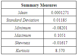
When analysing the return series plot (Figure 1), it is observed that the returns appear to be stabilised. They are clearly stationary with a common mean of 0. Extreme limits are set to 3 times the standard deviation away from their mean, assuming that 99.7% of the observations are from a normal distribution. It can be explicitly seen from the graph that a few points do lie outside the upper and lower limits of the boundary set, indicating the presence of large positive as well as large negative fluctuations in the returns. These large fluctuations provide evidence of extreme events in the US market. The plot also displays significant volatility clustering of the returns. Indeed, it is observed that periods of large returns are clustered and visibly distinct from those of small clustered returns. This suggests that heteroskedasticity is present in the series.

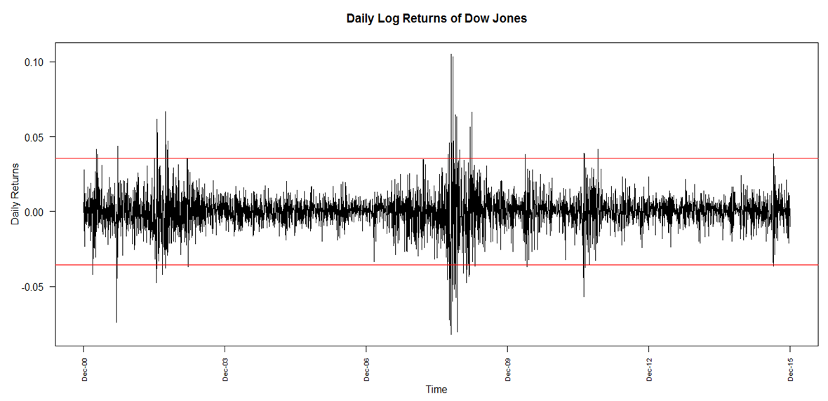Figure 1. Evolution of Daily Returns on Dow Jones

In order to confirm the presence of the different stylised facts present in the return series, the descriptive statistics of the new data set (Table 1) are also analysed. It is observed that the mean of the returns is almost 0, which is consistent with past findings on daily returns of financial time series. The minimum and maximum values are quite far from the mean, confirming the occurrence of extreme events during the time period. Moreover, as suggested in literature, the skewness is negative showing that the returns are slightly negatively skewed, probably due to presence of extreme values in the left tail of the return distribution. Furthermore, the kurtosis value is greater than 3, suggesting that the series is heavy-tailed, hence confirming the findings of Satchell & Knight [20]. The different characteristics of financial time series data as documented by numerous authors in literature, such as skewness, high kurtosis, sharp peaks (leptokurtosis) as well as volatility clustering are found present in this data set too. These allow to infer that the return series in fact exhibits departure from the normal distribution and is heavy-tailed.

Table 1. Descriptive Statistics of Daily Returns

Nevertheless, to further reaffirm the non-normality of the series, the normal Q-Q plot and the histogram of the return series are also analysed. The Q-Q plot (Figure 2) under the normal theoretical quantiles shows deviations from the 45^o line, which reasserts the assumption of fat-tailedness of the data. The histogram (Fig 3) is only slightly skewed, which implies that the distribution of the returns is not very heavy-tailed. Nevertheless, based on the other findings elaborated above, it would be justified to model the returns using a fat-tailed or a skewed distribution.

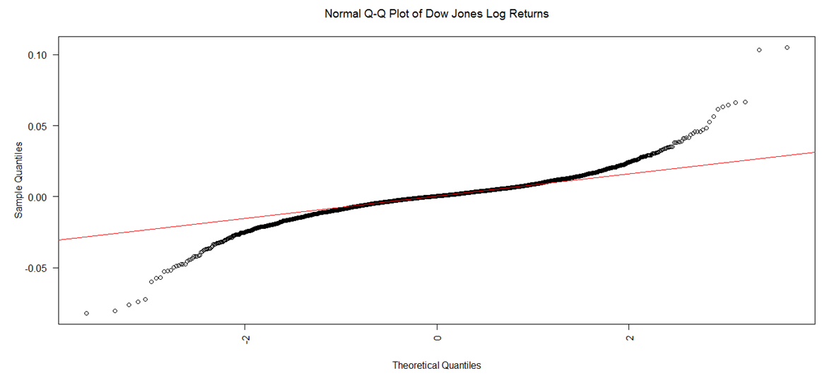Figure 2. Q-Q Plot of Daily Returns

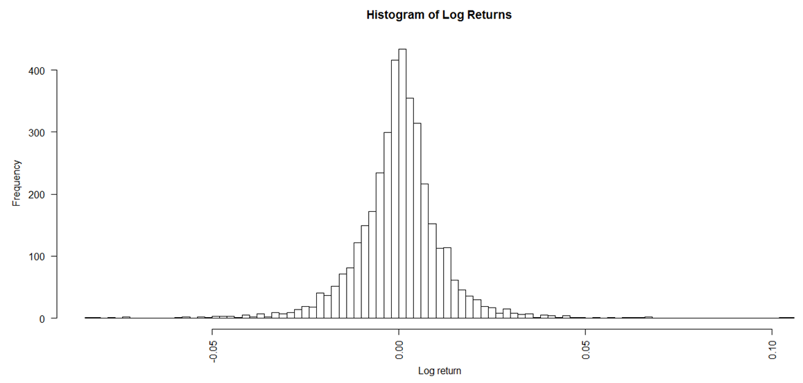Figure 3. Histogram of Daily Returns

The normality of the series can more formally be tested using the Jarque-Bera (JB) and the Shapiro-Wilk (SW) tests, to ensure that the skewness and kurtosis of the series indeed deviate from those of a normal distribution. Both JB and SW tests results obtained reject the null hypothesis of normality and add weight to the previous results. The p-values being almost equal to 0, give evidences that the sample data does not come from a normally distributed population.

2.2. Pre-fit Analysis

The autocorrelation function (ACF) and partial autocorrelation function (PACF) plots of the returns are examined in order to identify the GARCH conditional mean equation suitable for the data set. The ACF and PACF plots (Figure 4) show significant autocorrelation in the returns, although at some lags they appear weak. In addition, the ACF plots of the squared returns and the absolute returns (Figure 5) illustrate strong autocorrelation at almost all the lags. Squared returns can be used to measure the second order moment of the returns. Therefore, the squared returns ACF plot suggests that the variance of the returns conditional on past history may vary with time. Also, there is high persistence in both the squared and absolute returns and both demonstrate slow decay of the autocorrelations of squared and absolute returns respectively. The findings therefore confirm the presence of volatility clustering in the series and hence suggest that a combination of ARMA-GARCH may be appropriate. To ensure that ARCH-GARCH would indeed be relevant, Engle’s ARCH test is carried out. The corresponding p-value being close to 0 allows the rejection of the null hypothesis of no ARCH effects and hence provides further support to the use of GARCH in the modelling of the data series.

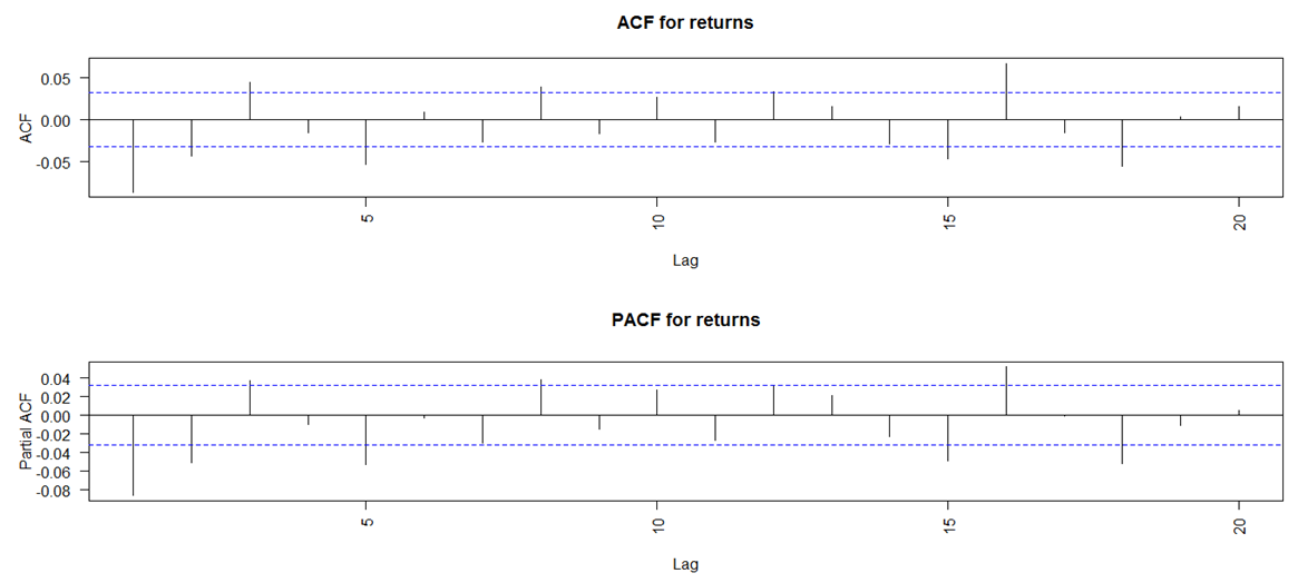Figure 4. ACF and PACF for Returns

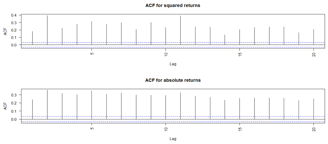Figure 5. ACF for Squared and Absolute Returns

2.3. Identifying the Conditional Mean Equation

It is desirable to choose a model with a mean equation that not only fits well but also has the least number of parameters, so as to limit the uncertainties in the forecast values. ARMA(m,n), AR(m) and MA(n) models with different lag choices can be fitted depending on the autocorrelation function (ACF) and partial autocorrelation function (PACF) plots obtained. In order to identify the best model, those values of m and n are chosen which minimise the model criteria AIC and maximise log-likelihood. ARMA(1,1) shows to be most parsimonious. It actually displays the lowest AIC value and the maximum log-likelihood value.

3. Methodology

Traditional GARCH modelling and Extreme Value Theory (EVT) approaches are now applied on the DowJones log returns to model Value-at-Risk (VaR) as a means for quantifying extreme market risk.

3.1. Model Specification

GARCH(1,1)

GARCH(1,1), which is the most commonly used process of all GARCH models, is implemented in this study. It is specified as follows:

where is a random variable denoting the mean corrected return/random shock. is a sequence of i.i.d. r.v. with mean 0 and variance equal to 1. The distribution of is conditional on all information available up to time . The dynamic behavior of the conditional variance is accounted by . This implies that , the conditional variance of today, is dependent on past squared disturbances, .

The effect of the distributional assumption on the variable is analysed, by using three distributions; namely the normal distribution, the t distribution and the skewed-t distribution introduced by Fernandez & Steel in 1998. The parameters are estimated using the Maximum Likelihood Estimation method, which is also called the conditional MLE. It is actually known to provide asymptotically efficient estimation of the parameters of the GARCH model.

EVT-POT

The Peak Over Threshold (POT) method consists of fitting the Generalised Pareto Distribution (GPD) to the series of negative log returns. Its main focus is the distribution of exceedances above a specified high threshold. For a random variable , the excess distribution function above a certain threshold is expressed as:

where represents the size of the absolute exceedances over . For , the excess distribution function can be rewritten as:

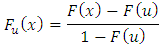From the above equation, the reverse expression which allows the application of POT-EVT can be deduced. It is given as follows:

There are two steps in the application of the POT method. Firstly, an appropriate threshold has to be chosen, beyond which the data points, which qualify as extreme events, are identified. GPD is then fitted to these data points to estimate the parameters of the distribution, which are finally used to calculate Value-at-Risk (VaR).

It is important to find the appropriate choice for the threshold of exceedances, u, beyond which data points are considered as extreme values. For choosing u, there is usually a trade-off between variance and biasness. As u becomes greater, more observations are used to estimate the parameters. Therefore, the estimates tend to have lower variation, hence lower variance. However, at the same time the limiting results of EVT may not hold, since deeper attention is given to the order statistics which may not contain relevant information. Consequently, this makes the estimators more biased.

The Hill plot proposes a graphical method for choosing an appropriate threshold by identifying the relevant number of upper order statistics. Hence, the Hill graph is basically a diagnostic plot for estimating the EVI. The graph plots Hill estimators against corresponding values of number of exceedances k. The appropriate threshold is usually the point at which the plot appears to be constant or stabilised. The Hill plot may not be practical for finding the appropriate threshold since the region of stability is not always obvious from the graph. As a result, more emphasis is given to MEF and Q-Q plots in this study. An appropriate threshold u would be the value from where the MEF exhibits a positive gradient, such that the exceedances follow a GPD with , provided the estimated parameters exhibit stability within a range of the selected u, [21]. The parameters of the GPD can be estimated in a number of ways, such as the MLE, Methods of Moments, Moment Estimation or Probability Weighted Moments. In this study, emphasis is given to the MLE and Moment Estimation methods. MLE is the most popular one but literature has shown that Moment Estimation also gives good results.

GARCH-EVT

The two-step procedure of McNeil & Frey [17] is investigated here. This method is especially useful when dealing with short horizon time periods. The two steps involved are summarised as follows:

Ÿ Estimate a suitable GARCH-type process and extract its residuals, which should be i.i.d.

Ÿ Apply Extreme Value Theory (EVT) to the obtained residuals in order to derive Value-at-Risk (VaR) estimates.

In this paper, filtering is firstly performed using the GARCH model with the symmetric t distribution since it adequately models fat-tailed series. EVT is then applied to the residuals, as elaborated above. This approach is usually known as conditional EVT technique, whereby both the dynamic GARCH structure and the residual process are taken into account.

3.2. Forecasting

After estimating the different model parameters and diagnosing the models, forecasting is carried out in order to compare the model forecasts with actual observations. The models are used to forecast 1-ahead daily VaR at both 95% and 99% confidence levels.

Value-at-Risk (VaR) Evaluation

There is a need to accurately estimate VaR, because the inaccurate estimation of this risk can have catastrophic repercussion in real life situations; for example inefficient allocation of capital can lead to serious implications on the stability and profitability of financial institutions. The overestimation of the risk can cause excess of capital requirements which may be unnecessary while the underestimation of it can lead to untimely exhaustion of capital. When using Generalised Autoregressive Conditional Heteroskedasticity (GARCH) modelling, VaR is calculated directly from the standard deviation obtained from fitting the distribution of returns. The relationship between the VaR and the standard deviation at time t can be expressed as follows:

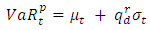For EVT-POT, VaR is calculated by using the following equation:

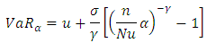Backtesting VaR

In order to measure the accuracy of the estimated risk, the risk models have to be backtested. Backtesting actually provides evidence of whether or not a risk model is reliable and accurate. Two popular statistical tests are used: firstly the unconditional coverage test, which takes into account only the frequency of the VaR violations and does not consider the time at which they occur, and secondly the conditional coverage test, which takes both factors into consideration.

Data Material

In this paper, the last 250 observations out of the 3762 daily returns are kept for forecasting and backtesting purposes. A rolling window forecast of 250 observations is actually used.

4. Estimation Results

This section analyses the forecasting performance of the three approaches; GARCH (with normal, t and skewed innovations), unconditional Extreme Value Theory (EVT) and lastly conditional EVT (combined GARCH with EVT). The comparative analysis is done on the basis of their backtesting performance.

4.1. Fitting Performance

4.1.1. Implementation of GARCH

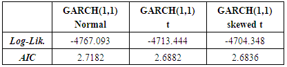
GARCH(1,1) with three innovations (normal, t and skewed-t) is fitted and, the log-likelihood as well as AIC values are obtained.

Table 2. Log-likelihood and AIC for GARCH with different innovations

The results show that the skewed-t distribution has the maximum log-likelihood and the minimum AIC values. However, not much difference between the three distributions is observed. It hence suggests that the skewed-t distribution only slightly outperforms both the normal and t distributions. The GARCH(1,1)-N model performs the least well. The results allow to deduce that innovations of fat-tailed distribution used to describe conditional distribution is justified. Skewed-t distribution, which accounts for both asymmetry and heavy tails, is probably the most suitable innovation to be modeled for this data set.

Parameter Interpretation

After the joint estimation of the variance and mean equations, the parameters of the models are obtained and analysed. It is observed that under different distributional assumptions, the parameters vary, implying that the distributional assumption does have certain effect on the estimation process. For the fat-tailed t distribution, the shape parameter is estimated, and for the skewed-t, both a shape parameter and a skewness parameter are obtained. The skewness parameter, having a very low p-value, is quite significant. Moreover, the shape parameters for both the t and skewed-t distributions are high, confirming the presence of heavy tails in the series. The results further show that the p-values of the GARCH parameters are very low, indicating that these parameters are also highly significant. It can thereby be inferred that there may not have been misspecification in the models.

4.1.2. Implementation of EVT

Threshold Selection

To find an appropriate value for the threshold, the MEF is analysed. From the graph (Fig 6), it can be observed that the graph is relatively constant between 0 and 1, implying that the threshold choice should be somewhere between 0 and 0.01 (1%). For the 20% exceedance, the threshold return is around 0.01, as shown in the graph. This further implies that the MEF may justify the use of 20% as threshold choice.

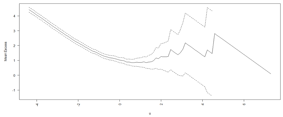Figure 6. Mean Excess Plot

Parameter Interpretation

Initially, only the first 250 data window is considered and is then approximated to the whole data series. The estimates of the Extreme Value Index (EVI) for the different exceedance percentage choices, that is 5%, 10%, 15% and 20% (12, 25, 37 and 50) are found using MLE and Moment Estimation. The results are obtained as follows:

Table 3. Estimators of EVI at different Exceedance Levels

In order to compare the EVI estimates of the two methods, graphs of the different estimators of the EVI at various exceedance levels are plotted (Figure 7).

Figure 7. Estimators of the EVI at different Exceedance Levels

The results show that the values of the EVI estimators are all positive, suggesting that the application of Peak Over Threshold (POT) would be appropriate. It can thereby be inferred that the tail index has a heavier tail behaviour than the exponential. The estimators are very reliable at all the exceedances level. However, it is wise not to consider the low levels of exceedances as possible thresholds, as this would involve very few observations for EVT to apply well. Therefore, 20% is preferentially chosen as an appropriate limit of the threshold. This means that for the first data window, 20% of 250 negative returns (which gives k = 50) would be considered as extreme values.

Model Validation

Q-Q plot is used to assess the reasonability of a Generalised Pareto Distribution (GPD) at the chosen 20% exceedance. The corresponding plot (Figure 8) is linear, providing evidence for the appropriateness of the GPD assumption at this exceedance. Moreover, to justify the use of GPD, the excess distribution plot and the plot of the tail distribution are also analysed (Figure 9). The plots show that exceedances lie close to the theoretical curves, showing a good fit.

In addition, the plot of the residuals is scattered with no visible trend present. Hence, the graphs support the use of GPD as the modelling distribution.

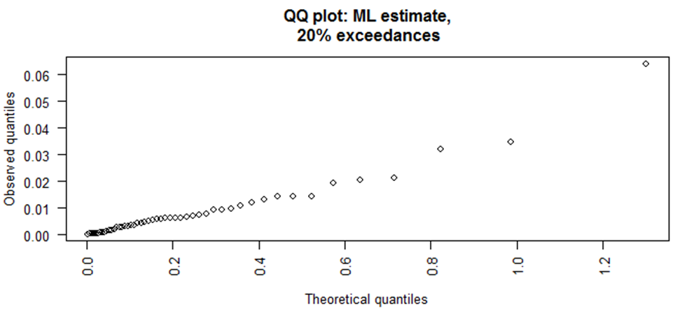Figure 8. Q-Q Plot at 20% Exceedance

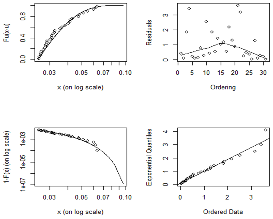Figure 9. Plots for appropriateness of GPD

POT-VaR over the Whole Series

Now, considering all the 3762 observations, EVT is applied to a moving data window of 250 days. The data is firstly transformed into negative log returns. A threshold of 20% is used in this analysis. The parameters are re-estimated every day based on the previous 250 days of observations. Since the MLE method is the most commonly used, it is preferentially used over the Moment Estimation to estimate the parameters of the Generalised Pareto Distribution (GPD). The parameters, and of the GPD are hence estimated using the MLE method. The graph (Fig 10) below illustrates the evolution of the EVI for the out-sample data window (last 250 data points) as estimated by MLE. The evolution of the parameter (Fig 11) is also plotted. Both graphs indicate that the parameters appear to be reliable over time. These are now used in the calculation of Value-at-Risk (VaR).

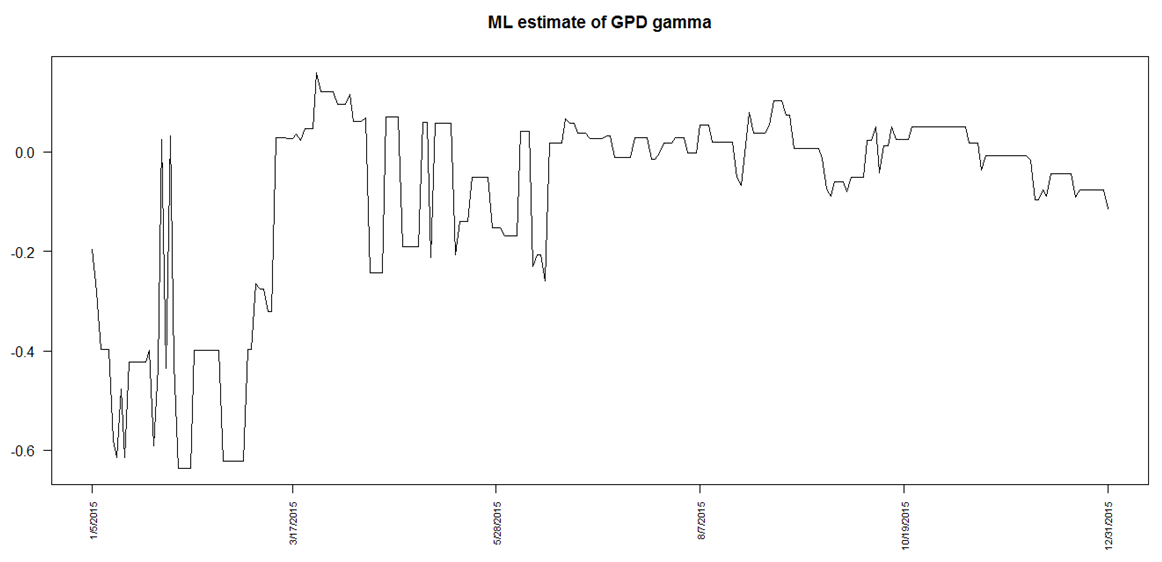Figure 10. Evolution of GPD parameter

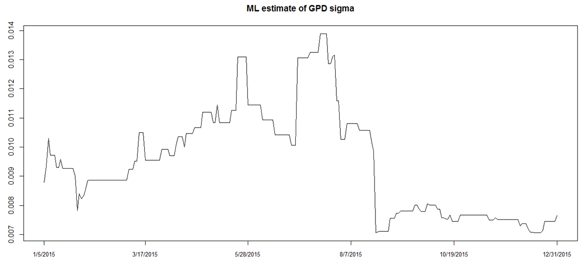Figure 11. Evolution of GPD sigma parameter

4.1.3. Implementation of GARCH-EVT

The residuals obtained from fitting GARCH to the series should be i.i.d. In order to verify the appropriateness of Extreme Value Theory (EVT) to these residuals, their descriptive statistics are analysed. The skewness (0.1065) and kurtosis (8.319) being quite large suggest that the application of EVT is admissible. EVT is therefore applied in the same way, as explained above, to obtain VaR-GARCH-POT estimates and finally the backtest tests results are obtained and analysed.

4.2. Value-at-Risk (VaR) Forecast

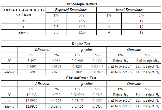
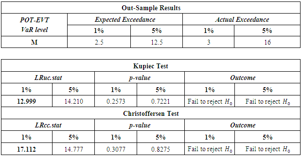
After estimating the parameters of the models and carrying out diagnostic checks, dailyVaR are now estimated. 1-step ahead VaR are forecasted and the models are re-estimated every one observation. This is done to ensure that the risk measure is more or less in conformity with actual practice. A series of 250 forecasts of Value-at-Risk (VaR) for one year is obtained. The 1-day ahead VaR is calculated at 95% and 99% confidence levels. Both levels of confidence are used for out-of-sample backtesting of VaR, in accordance to Basel II Backtesting Requirements, which stipulates that backtesting of VaR needs to be done on confidence levels other than 99%.

Usually, the smaller confidence level, the greater is the number of violations and easier it becomes to judge the forecasting performance of the model. This is why, at the 95% confidence level, it is expected to observe more violation points than at 99% level. A violation point is said to occur when the point lies below or above the true values of the returns. In this study, both confidence levels are considered so as to be able to investigate better the model accuracy when dealing with tails. At 99%, a lower portion of the tail is taken into consideration than at the 95%. The results are analysed using backtesting charts and quantitative statistical backtests.

4.2.1. Backtest Graphs and Results

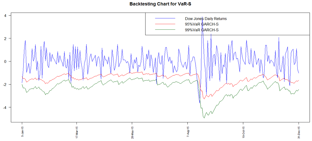
A graphical analysis is initially provided to illustrate an overall visual overview of the performance of the risk models at both 95% and 99% for all the models ie. GARCH Normal, GARCH t, GARCH Skewed t, POT and GARCH-POT.

All the graphs (Fig 12 to Fig 16) clearly display presence of VaR violations. The results obtained show that all the techniques adopted for VaR forecasting more or less fairly model downside risk. In addition to the backtest charts, a quantitative analysis, which is more reliable, is also provided. The number of VaR violations is counted and then compared to the expected number of losses at the chosen confidence level.

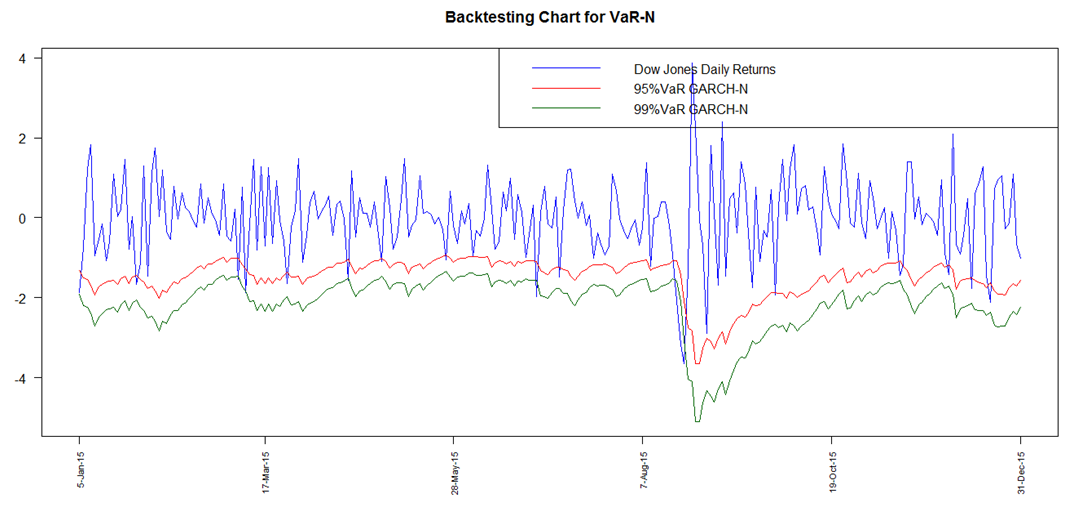Figure 12. Backtesting Chart for VaR GARCH Normal

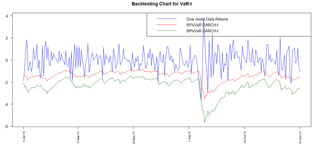Figure 13. Backtesting Chart for VaR GARCH-t

Figure 14. Backtesting Chart for VaR GARCH Skewed t

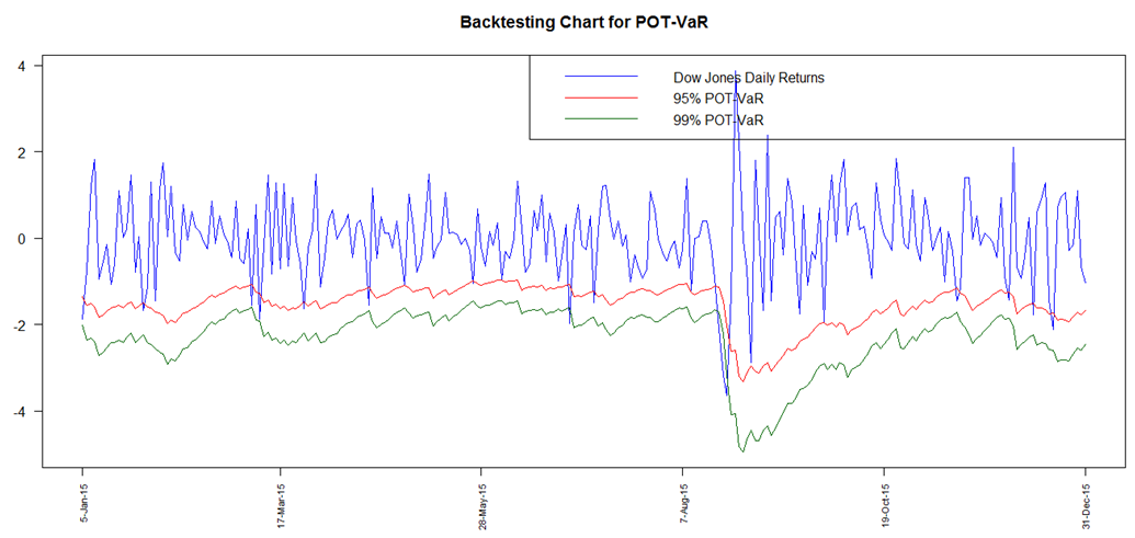Figure 15. Backtesting Chart for VaR-POT

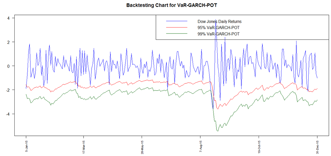Figure 16. Backtesting Chart for VaR-GARCH-POT

VaR-GARCH

For the GARCH models, all the innovations succeed in providing satisfactory results, except for the GARCH-N at 1% confidence level. The distribution of the skewed-t provides the best results. However, there is only slight difference in the values obtained for the different distributions. All the models pass the unconditional coverage test at the 5% exceedance, however at 1% exceedance, the GARCH-N fails the test. Furthermore, all the models pass the conditional coverage test at both the 1% and 5% exceedances, except again for the GARCH-N. This is anticipated since generally the normal distribution does not model tails quite accurately. Nevertheless, the number of VaR violations for all the GARCH innovations at both 95% and 99% levels of confidence are quite fair.

Table 4. GARCH Backtest Results

VaR-POT

Better results are obtained for the empirical application of unconditional EVT-POT approach to the data set as compared to the GARCH models. Both the unconditional and conditional coverage tests also provide better results (Table 5).

Table 5. POT-EVT Backtest Results

VaR-GARCH-EVT

The results obtained when GARCH is combined with EVT-POT is relatively the best compared to the other two techniques (Table 6). However, it can be seen that the results are only slightly improved. The unconditional as well as the conditional coverage tests are successfully carried out.

Table 6. GARCH-POT-EVT Backtest Results

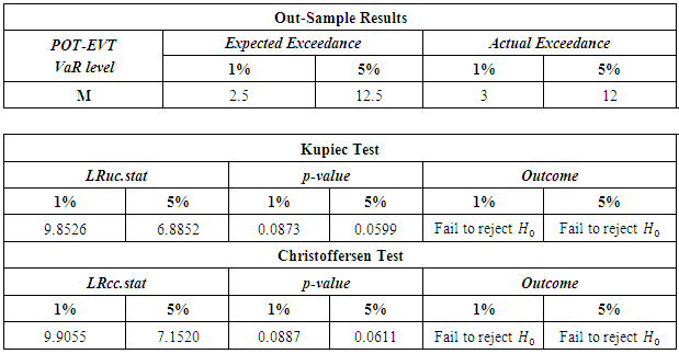
4.2.2. Comparative Analysis

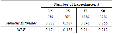
The failure rates for the GARCH models (normal, t and skewed t) as well as the unconditional and conditional EVT models, at the confidence levels of 95% and 99%, are tabulated, as shown below.

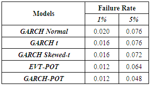The GARCH model performed quite well with all the innovations however the skewed-t distribution seemed to provide relatively superior results. At the 95% confidence level, the expected failure rate is 0.05 while at 99%, it is expected to be 0.01. The results show that the failure rates at both levels for all the models are relatively high than that expected. The GARCH-normal and GARCH-t failures rates as compared to the others are the highest and the same at 95%. This is quite unusual since generally the t is expected to perform better than normal. At both 95% and 99%, failure rates for both unconditional and conditional EVT are smaller. The results thus allow to deduce that EVT techniques (both conditional and unconditional) performed better as compared to the GARCH approaches, with conditional EVT (GARCH-POT) performing the best.

5. Conclusions

The main focus of this paper was to compare the forecasting power of different models in modelling Value-at-Risk (VaR), whereby the modelling adequacy of Generalised Autoregressive Conditional Heteroskedasticity (GARCH) and Extreme Value Theory (EVT) approaches were investigated. Three approaches were adopted namely [1] GARCH with normal, t and skewed-t innovations as well as [2] unconditional EVT and [3] conditional EVT. The empirical results reveal that in general, all the three approaches performed well in the measurement of extreme market risk.

The GARCH models using the fat-tailed and skewed distribution pass both the unconditional and conditional coverage tests meaning that the performance of the models was uniform over time. However, based on backtesting results of 1-day-ahead VaR predictions, the GARCH-N model fails to accept the hypothesis of correct coverage and independence at the 99% level. It is thus concluded that this GARCH innovation technique tends to underestimate risks during volatile periods, while overestimating risks during tranquil periods at this level. During these periods, EVT tends to perform better than traditional GARCH methods. The results obtained also indicate that GARCH combined with EVT to give conditional VaR estimates is the best technique to be considered for modelling of extreme market risk for financial data. It is indeed a reliable and powerful approach for modelling heavy-tailed distributions as argued by the findings of Kellezi & Gilli [22], Fernandez [10] and Gilli & Kellezi [8] among others, which concluded that EVT does give the most accurate estimates of VaR at higher confidence levels.

To conclude, the results showed that accounting for fat-tails and skewness using different distributions in both GARCH and EVT modelling produced more accurate and precise estimation of VaR forecasts. The more accurate the volatility specifications and forecasts are, the more they are likely to improve the quality of risk measures, leading to a successful implementation of risk management which is very important in management of downside risks.

Other variants and extensions of the GARCH model such as EGARCH, GJR-GARCH and TGARCH, that are capable to adequately incorporate properties like asymmetry and leverage effects respectively, can be used as an extension to this study. Furthermore, instead of using MLE for GARCH parameter estimation, Quasi-MLE which is asymptotically normal and consistent can be used for estimation of the GARCH parameters and current volatility before Extreme Value Theory (EVT) is applied to the residuals. Multivariate extension of the GARCH model such as the copula-GARCH may also be implemented to model Value-at-Risk (VaR).