1. Introduction

Employee attitude to work and their general job performance is dependent on the psychosocial characteristics of their working environment. These psychosocial characteristics which include status, promotion, decision making, and personal growth are variables that significantly affect the sense of empowerment felt by workers and determine the level of employees’ commitment and satisfaction to the work [1].

Previous studies by [2-4] have shown that job satisfaction is the perception and evaluation of an individual’s job over years and is dependent on demographic factors like age and gender.

Hence the aim of this study was however to model the relationship between age and job satisfaction using gamma distribution to ascertain the claim of non linearity relationship by past researchers with substantial mathematical and statistical evidence.

In statistical techniques, data transformation has been found very helpful as it improves the quality of model approximation and also makes inferences from such model to be robust [5, 6]. However, despite the importance of transformation, some imperfection in the parameter values of the approximate model compared to the raw data parameters, often times has always put a limit to the degree of asymmetry achieved [7]. This imperfection is such that if the original data were negatively skewed, then the transformation index shifts the transformed data mean position to the right to improve the degree of asymmetry and if the original mean position is skewed to the right, the transformed mean position is shifted inward to achieve approximate normality [5, 7]. Hence the choice of gamma (3P) distribution as assumed model is based firstly on the non normal nature of the variables and that normally distributed variables can be achieved by manipulating its parameter values. Secondly on the assumption that the imperfection noticed as a result of shift in the mean (location) position due to transformation can be estimated from the location parameter and finally that the transformation has no effect on the variance of the distribution since the Box-Cox transformation engaged is a variance stabilizing transformation. A proper Jacobean transformation between the power transformation function and the assumed model was ensured to correct the distortion in the original measurement scale and ease interpretation of result. See [5, 6, 8] on Box-Cox transformation and [9] for the properties of gamma distribution.

2. Literature Review

The power transformation of data to achieve approximate normality and enhance statistically based inference has been shown to be of great importance in the last five decades [6, 8]. Of all these power transformations, Box-Cox transformation defined by 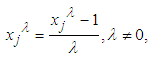or 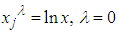is the most popular. However, most statistician prefers to obtain the value of at which the expression 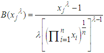has the minimum variance. For each j = 1,2,......n, the variance value of the function is obtained for each The minimum of all the variances and its associated is desired [5-8].

Note that in gamma (3P);

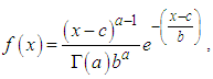
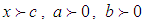1. The location parameter c could be positive or negative depending on the shift direction leading to a transformation variable or respectively.

2. The value of parameter and will determine if the variable can be fitted with gamma 3P, gamma 2P or the standard normal density.

In situation when the original data is approximately normally distributed, there is no need for transformation and so The distribution thus reduces to a gamma (2P) Then if the shape parameter is large and the scale parameter the variable is approximately distributed as standard normal random variable [9].

3. Material and Data Collection

Two self administered questionnaires was used to capture the required information for the study. A self developed questionnaire was used to obtain the demographic variables such as age, sex, marital status and so on. The job satisfaction of respondent was measured using the Minnesota Satisfaction Questionnaire (MSQ). MSQ was developed by the Vocational Psychological Research unit of the University of Minnesota in 1967 and it has a reliability coefficient of 0.90. A total of 393 teachers from different secondary schools within Abeokuta the Ogun state capital in Nigeria were used in the study. Necessary ethical approvals were obtained before the commencement of the study.

4. Methodology

• Deriving the composite gamma-power function for bi-variate relationship using Jacobean transformation.

• Transformation of both job satisfaction and age to achieve normality via Box-Cox techniques.

• Estimating the parameters of the gamma distribution using moment estimation method.

• Hypothesis testing of the fitted models using kolmogorov-smirnov test (KS).

• Plotting Job satisfaction against Age using codes written with R.

5. Result

Deriving the composite gamma-power function and its joint probability density function

The proper Jacobean transformation for a transformed variable can be derived as 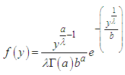where. can be shown to be a probability density function. The parameters and can be obtained from the moment estimates of the model. is the transformation index from Box-Cox.

Suppose we have two successfully transformed variables and then the joint density model of the two random variables is given as

.

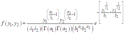Lets define a ratio bi-variate relationship between and then if and then

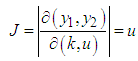and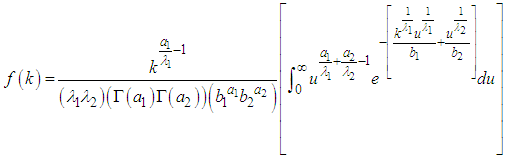

Note that the function can be simplified further via parameter manipulations, or else the integral part will be solved by numerical integration. However given that and are job satisfaction scores and age respectively then k is measure of job satisfaction growth rate with age.

6. Discussion of Result

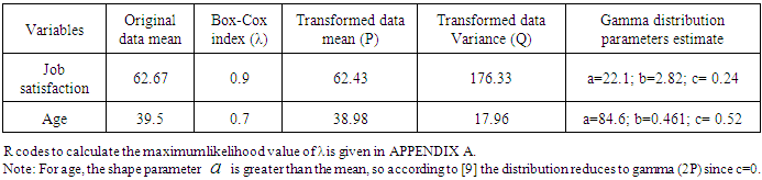
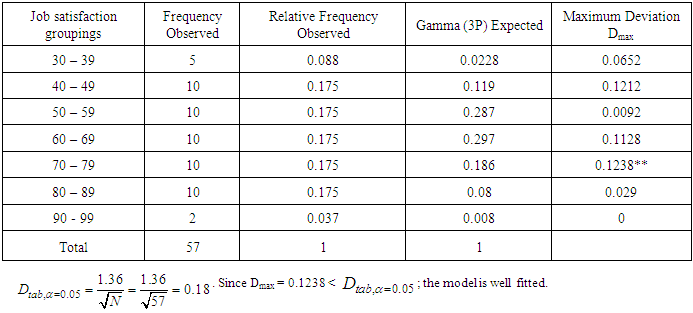
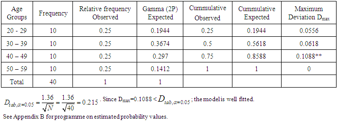
The condition that the shape parameter is greater than the mean and the scale parameter b is within the range determines our assumption of assumed normal or non normal distribution for any of the variables and the need for transformation technique to improve normality. In case of non normality, the numerical value of the location parameter was used as the measure of shrinkage or spread required to shift the data towards the mean. Table 1 gives the summary of the transformation index and the parameter values of the distribution fitted for each variable. The evidence of model fitness for non repeated responses was ascertained in Table 2 using kolmogorov smirnov test (KS).

Table 1. Summary of the transformation index value and the distribution parameter values

Table 2a. Kolmogorov-Smirnov test for goodness of fit on Job Satisfaction groupings

Table 2b. Kolmogorov-Smirnov test for goodness of fit on Age groupings

The composite gamma-power probability density function for job satisfaction growth rate with age (k) was obtained as Codes were written in R to evaluate (Appendix C).

A scatter plot of the job satisfaction growth rate to the ages of respondents gave a U shape (figure 1). Freshly employed staffs, within the age of 20-25 years has a high level of job satisfaction within 80-120 percent; possibly because they just got a new job upon which they can develop their career in the mist of high unemployment rate. A reason why careful selection of career is of great important. As the respondents age moves from 25-30 years, the level of job satisfaction drops to 40% and continues to drop till it becomes stable at 10% between the age brackets of 33-44 years. A job satisfaction of 10% is very low. However beyond 45 years of age, the respondents’ job satisfaction begins to pick up at a very slow rate. The continues decrease in job satisfaction from ages 20-30 years till it becomes stable between age brackets 33-44, may be due to the fact that as people grow older with this career, personality and situational factors set into play and these may determine the desire to go on with this career or not. Personality factors include risk taking tendency and sense of control over one’s destiny. While, situational factor include increasing disenchantment with one’s present career, discovery of other occupation that promises a greater satisfaction and pivotal events (divorce, death of a loved one) that lead one to shift life goals and priorities. These factors may determine the satisfaction one gets from this career and the desire to stay on with the career. The level of job satisfaction growth rate increases noticeable as respondents attained the age of 50 years and beyond. The respondents within the age bracket of 50-60 years of age, has a high level of job satisfaction between 60-120 percent with sharp job satisfaction growth rate. This may result from the fact that as one gets older above the average age; the rise in job satisfaction could come from reduced aspirations due to the recognition that there are few alternative jobs available once their careers are established [11].

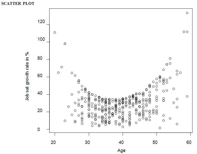Figure 1. The graphical relationship between Job satisfaction growth rate and Ages of teachers in secondary schools across Abeokuta. (See Appendix C for the R codes used for the scatter plot.)

7. Conclusions

The assumption of normality and the need for power transformation was checked using the parameter values of gamma distribution. The composite function for job satisfaction growth rate was plotted against the age in a scatter plot (Figure 1). We observed a non-linear relationship between age and job satisfaction. The non-linearity shows a U-shaped relationship, with those in the very young and old age groups being the most satisfied. This illustrates that as age increases from 33 years to 40 years, the job satisfaction levels decreases. This reduction in the job satisfaction level continues until around the age of 40-44 years, after which any further increase in age beyond 44 years shows a corresponding increase in the job satisfaction level.

Appendix

APPENDIX A:- Codes to obtain Box-Cox transformation index

> z <- c(31, 34, 35, 36, 37, 38, 39, 40, 42, 43, 45, 46, 47, 48, 49, 50, 51, 52, 53, 54, 55, 56, 57, 58, 59, 60, 61, 62, 63, 64, 65, 66, 67, 68, 69, 70, 71, 72, 73, 74, 75, 76, 77, 78, 79, 80, 81, 82, 83, 84, 85, 86, 87, 88, 89, 90, 92)

> K <- seq (-1, 1.5, by =0.1)

> A <- (prod (z))^(1/(length (z)))

> a <- (((z^-1)-1)/(-1*(A^-2)))

> b <- (((z^-.9)-1)/(-.9*(A^-1.9)))

> c <- (((z^-.8)-1)/(-.8*(A^-1.8)))

> d <- (((z^-.7)-1)/(-.7*(A^-1.7)))

> e <- (((z^-.6)-1)/(-.6*(A^-1.6)))

> f <- (((z^-.5)-1)/(-.5*(A^-1.5)))

> g <- (((z^-.4)-1)/(-.4*(A^-1.4)))

> h <- (((z^-.3)-1)/(-.3*(A^-1.3)))

> i <- (((z^-.2)-1)/(-.2*(A^-1.2)))

> j <- (((z^-.1)-1)/(-.1*(A^-1.1)))

> k <- (A*log (z))

> l <- (((z^.1)-1)/(.1*(A^-0.9)))

> m <- (((z^.2)-1)/(.2*(A^-0.8)))

> n <- (((z^.3)-1)/(.3*(A^-0.7)))

> o <- (((z^.4)-1)/(.4*(A^-0.6)))

> p <- (((z^.5)-1)/(.5*(A^-0.5)))

> q <- (((z^.6)-1)/(.6*(A^-0.4)))

> r <- (((z^.7)-1)/(.7*(A^-0.3)))

> s <- (((z^.8)-1)/(.8*(A^-0.2)))

> t <- (((z^.9)-1)/(.9*(A^-0.1)))

> u <- (((z^1.0)-1)/(1.0*(A^-0.0)))

> v <- (((z^1.1)-1)/(1.1*(A^0.1)))

> w <- (((z^1.2)-1)/(1.2*(A^0.2)))

> x <- (((z^1.3)-1)/(1.3*(A^0.3)))

> y <- (((z^1.4)-1)/(1.4*(A^0.4)))

> z <- (((z^1.5)-1)/(1.5*(A^0.5)))

> K1 <- c(var (a), var (b), var (c), var (d), var (e), var (f), var (g), var (h), var (i), var (j), var (k), var (l), var (m), var (n), var (o), var (p), var (q), var (r), var (s), var (t), var (u), var (v), var (w), var (x), var (y), var (z)).

APPENDIX B:- Code to estimate the probability values of job satisfaction and age

> Job <- c(31, 34, 35, 36, 37, 38, 39, 40, 42, 43, 45, 46, 47, 48, 49, 50, 51, 52, 53, 54, 55, 56, 57, 58, 59, 60, 61, 62, 63, 64, 65, 66, 67, 68, 69, 70, 71, 72, 73, 74, 75, 76, 77, 78, 79, 80, 81, 82, 83, 84, 85, 86, 87, 88, 89, 90, 92)

> Age <- c(20, 21, 22, 23, 24, 25, 26, 27, 28, 29, 30, 31, 32, 33, 34, 35, 36, 37, 38, 39, 40, 41, 42, 43, 44, 45, 46, 47, 48, 49, 50, 51, 52, 53, 54, 55, 56, 57, 58, 59)

> x <- c(31, 34, 35, 36, 37, 38, 39, 40, 42, 43, 45, 46, 47, 48, 49, 50, 51, 52, 53, 54, 55, 56, 57, 58, 59, 60, 61, 62, 63, 64, 65, 66, 67, 68, 69, 70, 71, 72, 73, 74, 75, 76, 77, 78, 79, 80, 81, 82, 83, 84, 85, 86, 87, 88, 89, 90, 92)

> b <- 2.824

> a <- 22.10

> c <- 0.24

> f <- ((x-c)^(a-1))*(exp (-((x-c)/b)))/((gamma (a))*(b^a))

> i <- f/sum (f)

x non repeated response of job satisfaction

> y <- c(20, 21, 22, 23, 24, 25, 26, 27, 28, 29, 30, 31, 32, 33, 34, 35, 36, 37, 38, 39, 40, 41, 42, 43, 44, 45, 46, 47, 48, 49, 50, 51, 52, 53, 54, 55, 56, 57, 58, 59)

> e <- 3.46

> d <- 11.42

> h <- 0

> g <- ((y-h)^(d-1))*(exp (-((y-h)/e)))/((gamma (d))*(e^d))

> j <- (g/sum (g))

y non repeated response of respondents age.

APPENDIX C: Code to obtain the scatter plot

Job > z1 <- c(74, 78, 74, 52, 82, 75, 79, 69, 66, 65, 66, 67, 72, 61, 69, 69, 69, 69, 69, 65, 69, 66, 69, 62,69, 71, 68, 73, 68, 73, 71, 59, 72, 67, 58, 79, 61, 74, 65, 70)

Age > z2 <- c(20, 21, 22, 23, 24, 25, 26, 27, 28, 29, 30, 31, 32, 33, 34, 35, 36, 37, 38, 39, 40, 41, 42, 43, 44, 45, 46, 47, 48, 49, 50, 51, 52, 53, 54, 55, 56, 57, 58, 59)

> a1 <- 22.10

> b1 <- 2.824

> k1 <- 0.9

> a2 <- 11.42

> b2 <- 3.46

> k2 <- 1

> x <- (z1^k1)

> y <- (z2^k2)

> job <- (1/k1)*(Job^((a1/k1)-1))*(exp (-((Job^(1/k1))/b1)))/((gamma (a1))*(b1^a1))

> Age1 <- (1/k2)*(Age^((a2/k2)-1))*(exp (-((Age^(1/k2))/b2)))/((gamma (a2))*(b2^a2))

> jobage <- (job/Age1)*100

> plot (Age, jobage)