George M. Matiri1, Kennedy L. Nyongesa2, Ali Islam1
1Department of Mathematics, Egerton University, Nakuru, Kenya
2Department of Mathematics, Masinde Muliro University of Science and Technology, Kakamega, Kenya
Correspondence to: George M. Matiri, Department of Mathematics, Egerton University, Nakuru, Kenya.
| Email: |  |
Copyright © 2017 Scientific & Academic Publishing. All Rights Reserved.
This work is licensed under the Creative Commons Attribution International License (CC BY).
http://creativecommons.org/licenses/by/4.0/

Abstract
The concept of pool testing originated with Dorfman in the context of blood testing as an economical method of testing blood samples of army inductees in order to detect the characteristic of interest. Apart from classification problem, pool testing can also be used in estimating the prevalence rate of a trait in a population which was the focus of our study. In approximating the prevalence rate, one-at-a-time testing is time consuming, expensive and is bound to errors hence pool testing procedures have been proposed to address these problems. Despite these procedures, when pool testing strategies are used using imperfect kits, there tend to be loss of sensitivity. Lost sensitivity of a test is recovered by retesting pools classified positive in the initial test. This study has developed statistical model which is used to consecutively choosing some combination of the three experiments namely: one–at-a-time, pooled testing and pooled testing with retesting of the positive pools for estimating the prevalence rate of a trait with imperfect tests. The experiments are selected sequentially, so that at each stage, the information available at that stage is used to determine which experiment to carry out at the next stage. The method of maximum likelihood estimator (MLE) is used in obtaining the estimators. The Fisher information for each of the three experiments is compared and the cut-point values where one experiment is better than the other are computed. Properties of the estimators are discussed and compared and the joint model is found to be more efficient.
Keywords:
Proportion, Proportion estimation, Group, Group testing, Cut off Value, Sensitivity, Specificity
Cite this paper: George M. Matiri, Kennedy L. Nyongesa, Ali Islam, Consecutively Choosing between Three Experiments for Estimating Prevalence Rate of a Trait with Imperfect Tests, International Journal of Statistics and Applications, Vol. 7 No. 2, 2017, pp. 93-106. doi: 10.5923/j.statistics.20170702.04.
1. Introduction
In many applications, units can be classified as defective or non defective. Pool testing involves pooling such units into groups or pools, testing the groups, and classifying each group as defective or non-defective. A group is defined as non-defective if non of the unit in the group contains the characteristic of interest otherwise a group is said to be defective. A group testing design has been shown to be a compelling alternative to one-at-a-time testing in many areas where rare traits are of interest. Research has shown that pool studies can be used in plant pathology, genetics and reduction of cost in early stages of drug discovery (Hammick and Gastwirth, 1994; Swallow, 1985; Xie et al., 2001). Pool testing has also been applied in screening the population for the presence of HIV antibody (Kline et al., 1989 and Manzon et al., 1992). Computational testing that focuses on classifying subjects has been developed Maheswaran et al. (2008). Recently more research work are focused on estimating the rate of trait. Thomson (1962) considered estimation problem using pool testing which was later considered by Brookmayer (1999) by introducing errors. Sufficiently accurate estimate of the prevalence can be obtained from testing pooled samples as demonstrated by Hammick and Gastwirth (1994) and their procedure provides greater protection of respondent’s identity which can be useful in improving the response rate. On the same year, Gastwirth and Johnson (1994) used pool testing to estimate HIV prevalence cost-effectively. Hardwick et al., (1998) considered sequentially deciding between two experiments for estimating a common success prevalence rate where he considered the individual Bernoulli trials or the product of k individual independent Bernoulli trials. Nyongesa (2011) used moment method to estimate the prevalence and he observed that his proposed testing procedure reduced misclassification, particularly the false positives. Computational statistics has been used in pool testing to compute the statistical measures when perfect and imperfect tests are used (Syaywa and Nyongesa, 2010; Tamba et al., 2012). Benefits from group testing depend on size of the pools. Swallow (1985) showed that large group sizes can lead to estimators with enormous bias. In addition, there are biological issues to be considered. For example in HIV testing, enzyme-linked immunosorbent assay tests (ELISA) are commonly used in screening experiments to detect the presence of the virus. However, sensitivity levels for such tests are known to be poor when many blood samples are pooled together. With many of the standard enzyme-linked immunosorbent assay tests (ELISA), group sizes of up to 15 are typically used without experiment dilution effects (Behets et al., 1990; Cahoon-Young et al., 1989; Kline et al., 1989; Tu al., 1995). Recent studies have provided algorithm for the computation of pool sizes (Ding and Xiong, 2015). This study has focused on estimation of proportions and in particular a better estimation of the prevalence rate. The essence of the study, is to device a method of selecting between three experiments namely: i) individual testing of items of a population with a view to estimating prevalence rate p, with misclassification, this experiment will be denoted by 1E,ii) pool testing experiment as proposed by Dorfman (1943) but with errors in inspection, this experiment will be denoted by 2E and iii) estimating the prevalence rate of the characteristic of interest by retesting the pools declared positive in the first pool test and this experiment will be denoted by 3E. The rest of the paper is arranged as follows: in Section 2 we shall develop the models and formula for calculating Fisher information, in Section 3 we shall plot the graphs Fisher information against the value of p. In Section 4 we shall compute the cut off values. In Section 5 we shall develop the joint model and in section 6 we shall compute the MLE of p of the joint model. In section 7 we shall compare the variances of the models by plotting their graphs. In Section 8 we shall compute the ARE values and in section 9 we shall have conclusion of the study.
2. The Model
The model have been split into three, that is 1E-, 2E-, and 3E-experiments. r, s and t have been assumed to be the total number of observations from 1E-, 2E-, and 3E-experiments respectively. In typical sequential allocation problems, different experiments give information about different parameters. However, in this study, the three experiments i.e 1E-, 2E-, and 3E-experiments give information about the same parameter (p), although one experiment have given more information than the other two experiments under consideration depending on the actual value of the parameter, pool size, sensitivity and specificity of the tests. For simplicity, it has been assumed that individual units being pooled are independent and identically distributed Bernoulli random variables.
2.1. The 1E-experiment
If 1E-experiment is to be used to estimate the prevalence rate  , and if
  for
for  is a sequence of identically independent distributed random variable, then
 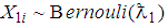 where
where  is the probability of declaring an individual as positive defined by the relation,
 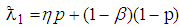 given
given  and
and  are sensitivity and specificity of the tests respectively.For a single experiment, the probability density function is
 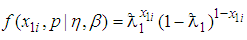 | (1) |
The Fisher information denoted by  , on the prevalence rate
  contained in a single observation of the 1E-experiment is
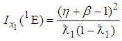 | (2) |
easily obtained by MLE method from (1). If  observations from only the 1E-experiment are used to estimate
  , then the maximum likelihood estimator of p, denoted by
  is
is 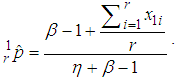 | (3) |
The asymptotic variance of  is obtained from (2) which yields
 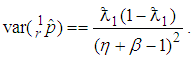 | (4) |
2.2. The 2E-experiment
The 2E-experiment involves putting together items to form a pool and testing the pool rather than testing each individual for the evidence of a characteristic of interest. A negative reading indicates that the pool contains no defective item and a positive reading indicates at least one defective item in the pool. Pooling procedures have proved to reduce the cost of testing when the prevalence rate is low. In this experiment, the probability of declaring a pool of size  positive is denoted by
 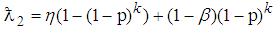 . If
. If  denote a sequence of identically independent distributed random variables for
  then
then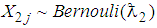 . For a single experiment equivalently the probability density function is
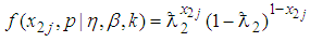 | (5) |
and the Fisher information denoted by  contained in a single observation of the 2E-experiment is
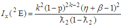 | (6) |
Suppose there are  pools for the 2E-experiment each of size k, available for estimating
  and suppose
  pool test positive on the test, then the maximum likelihood estimator of p, denoted by
  is
is 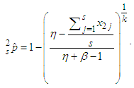 | (7) |
Noted is Thompson (1962) maximum likelihood estimator (MLE) of p i.e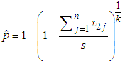 is a special case of (7).The asymptotic variance of
  is
is 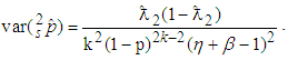 | (8) |
2.3. The 3E-experiment
The 3E-experiment involves retesting of the pools declared positive in the first pool test inorder to approximate the prevalence rate. Retesting of already tested pools reduce misclassification (Nyongesa, 2011). In this experiment, the probability of declaring a pool of size  positive is denoted by
  where
where 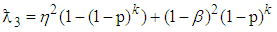 . If
. If  denote a sequence of identically independent distributed random variables for
  , then
  . For a single experiment the probability density function is
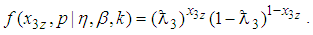 | (9) |
Similarly the Fisher information contained in a single observation of the 3E-experiment is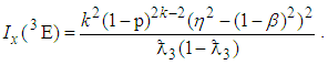 | (10) |
If t observations from the 3E -experiment are used to estimate  and
and  pool tests positive, then the maximum likelihood estimator of p, denoted by
  is
is 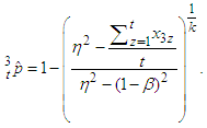 | (11) |
Equivalently the asymptotic variance of  obtained from (10) is
 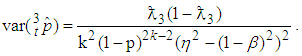 | (12) |
3. Comparison of  of 1E-, 2E- and 3E-experiments
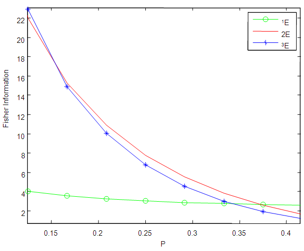
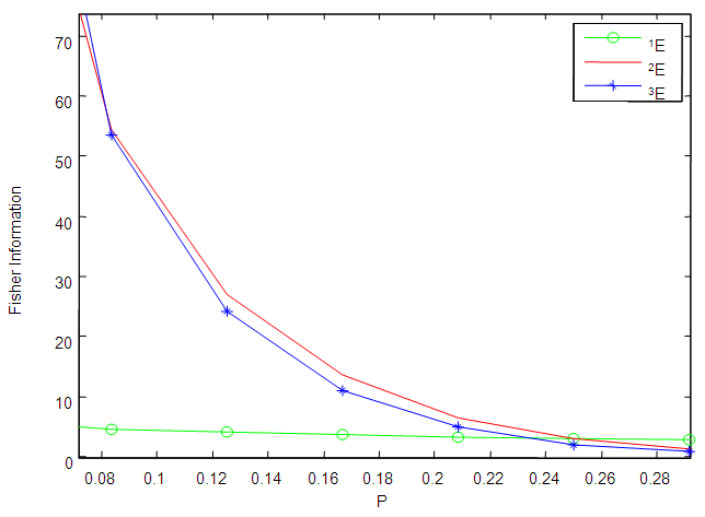
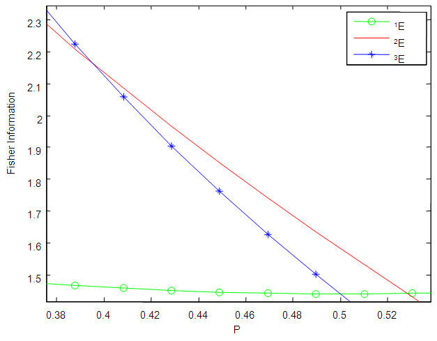
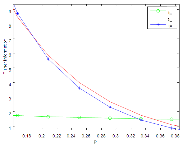
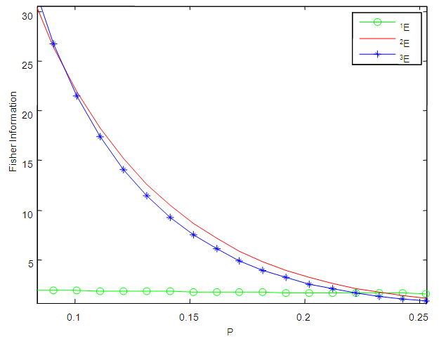
This study compares the Fisher information of 1E-, 2E- and 3E-experiments in this section by plotting the graphs of  of 1E-, 2E- and 3E-experiments for values of
 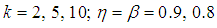 versus
  As seen from Figures 1 to 6, the Fisher information for the 1E -experiment is independent of the pool size hence it is not affected by change of the value of
  For the 2E - and 3E-experiments, the Fisher information is very high for small values of
  and it approaches zero as
  increases. As sensitivity and specificity of the test kits increases, the gap between the Fisher information of the 2E - and 3E -experiments shrinks. Holding
  constant, increasing sensitivity and specificity of the test kits, the region at which the Fisher information of the 1E- and 3E-experiments is better shrinks while for 2E-experiment increases. Similarly as
  increases the region in which the Fisher information of 1E - and 3E-experiments is better decreases while that of 2E-experiment increases. From Figures 1 to 6 it can be concluded that the 3E-experiment is better than 1E- and 2E-experiments for values of
  relatively small, for values of
  relatively large, the 1E-experiment is better and the 2E-experiment is better for some values of
  between 0 and 1. It is also noted that the region in which one experiment is better than the other experiments depends on sensitivity, specificity and the pool size.
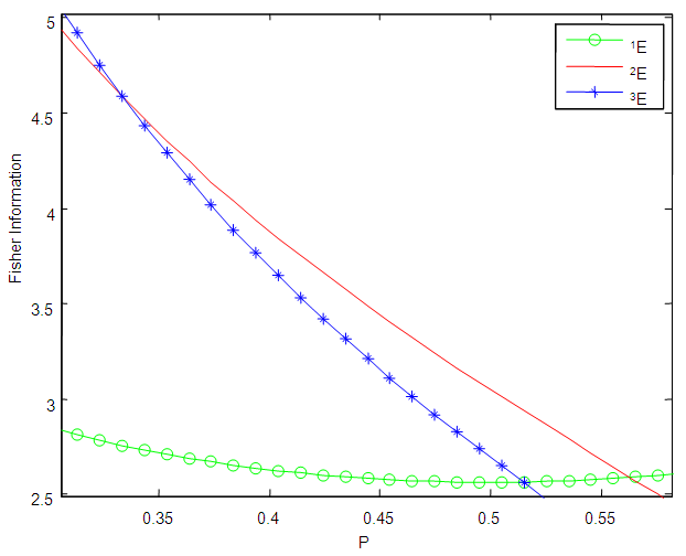 | Figure 1. A plot of Fisher information against the value of  with with  and and  |
 | Figure 2. A plot of Fisher Information against the value of  with with  and and  |
 | Figure 3. A plot of Fisher information against the value of  with with  and and  |
 | Figure 4. A plot of Fisher Information against the value of  with with  and and  |
 | Figure 5. A plot of Fisher Information against the value of  with with  and and  |
 | Figure 6. A plot of Fisher Information against the value of  with with  and and  |
4. Computation of Cut-Point Values
The cut-point value is defined as the value of p at the point where the Fisher information of one of the experiment surpasses the Fisher information of the other experiment while comparing any two of the 1E-, 2E- and 3E-experiments. If  is the cut-point value, then
  is a unique root in [0, 1] of the equation
  for
for 
 and
and 
4.1. Computation of Cut-Point Values of  and
and 
In this section the cut-point values of 1E- and 2E-experiments are computed by equating the Fisher information of the two experiments. Therefore equating (2) and (6) and simplifying yields | (13) |
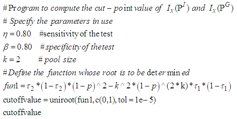
(13) has no solution in closed form therefore the equation is solved iteratively using an R code that we developed which is presented in Appendix A.
4.2. Computation of Cut-Point Values of  and
and 
The cut-point values of 1E- and 3E-experiments are computed in this section by equating (2) and (10) which yields | (14) |
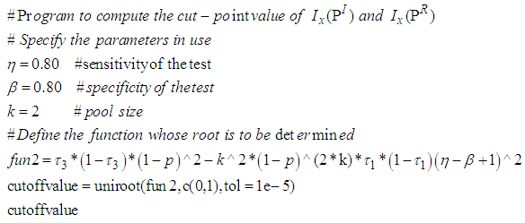
after simplifying. Similarly (14) is solved iteratively using an R code that we developed presented in Appendix B.
4.3. Computation of Cut-Point Values of  and
and 
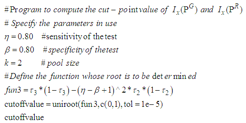
Similarly the cut-point values of 2E- and 3E-experiments are computed by equating (6) and (10) which yields 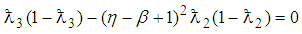 | (15) |
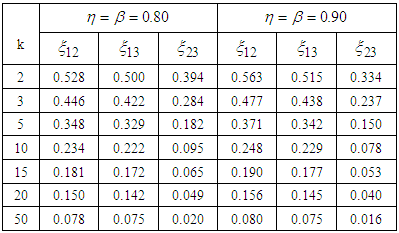
after simplifying. Equivalently (15) is solved iteratively using an R code developed which is presented in Appendix C.For various values of  and
and  the values
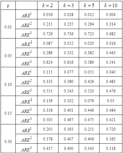
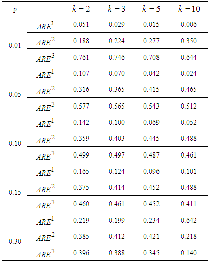
  the roots of (13), (14) and (15) are given in Table 1.From Table 1 it can be noted that the cut-point values are sensitive to k (pool size). As specificity and sensitivity increases the cut point value between 1E- and 3E-experiments increases while that between 2E- and 3E-experiments decreases. It is observed from Table 1 that as the pool size (k) increases, keeping
  and
and  the same, the region in which the 3E-experiment is better than the 2E- and 1E- shrinks. Increase in sensitivity and specificity leads to decrease of the area which 1E- and 3E -experiments is better than 2E-experiment. In general the exact values of p where one experiment is better than the others depends on the pool size (k), sensitivity
  and specificity
  of the tests.
Table 1. Cut-point point values for various values of

 |
| |
|
For example if  k = 3 and N tests are available, then the allocation that maximizes the information about
  is:
is: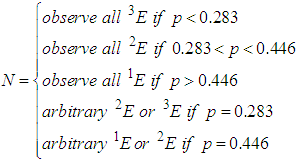 In general, if N tests are available, then the allocation that maximizes the information about
  is
is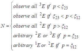 Note also that the region where one experiment is better than the other depends on the unknown parameter
  hence adaptive rule is suggested where
  is estimated at each stage and the next observation is allocated depending on the relationship between the estimated
  and the cut-point value.
5. The Joint Model
If r, s and t are the total number of observations from 1E-, 2E- and 3E-experiment respectively, then the joint probability density function of the random variables  and
and  from the 1E-, 2E- and 3E-experiments respectively is a multinomial probability density function. The joint probability density function is given by the product of their respective density functions, since the random variables are assumed to be independent, therefore
 | (16) |
The joint likelihood function of (16) is | (17) |
Taking logarithm on both sides of (17) and differentiating with respect to  yields
 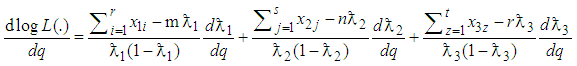 | (18) |
where 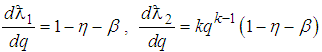 and
and 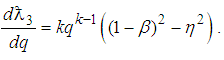 Equating (18) to zero leads to
 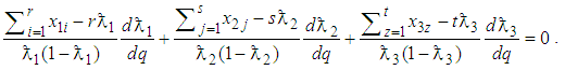 | (19) |
The only variable in (19) is  Hence
Hence 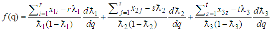 | (20) |
is a function of  which can be solved iteratively. The value of
  computed from (20) is denoted by
  hence the maximum likelihood estimator of p, denoted by
  of the joint model is
  The asymptotic variance of
  is obtained by solving
  where
where  is the joint probability density function given by (16). Therefore
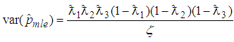 | (21) |
where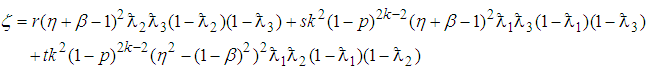
6. Estimator of Prevalence Rate, Its Variance and Confidence Interval
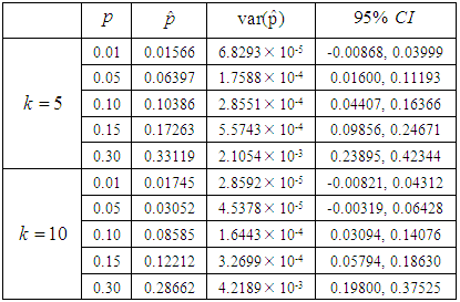
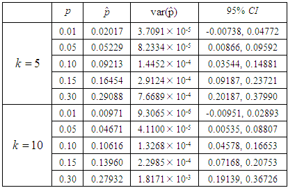
The maximum likelihood estimator  of the prevalence rate of the joint model, the variance and 95% Wald-type confidence interval of the MLE for values of
  and
and  are computed in this section.From Tables 2 and 3 it is observed that the maximum likelihood estimators of the prevalence rate are very close to the actual value which were used to simulate the estimators. The population estimators resulting from the experiments are used to evaluate the
  confidence limits of the confidence interval of the simulated estimators where
  is the level of significance and it is noted from Tables 2 and 3 that the actual value is within the limits.
Table 2. Maximum likelihood estimator, variance and Confidence interval for different values of p for
 and and

 |
| |
|
Table 3. Maximum likelihood estimator, variance and Confidence interval for different values of p for
 and and

 |
| |
|
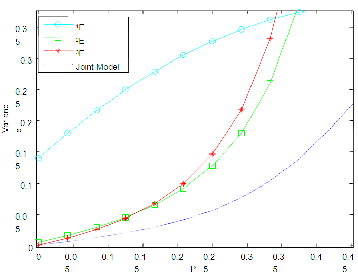
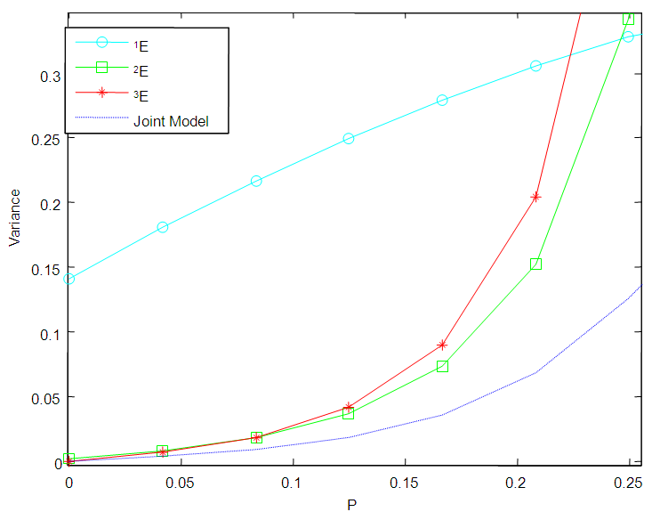
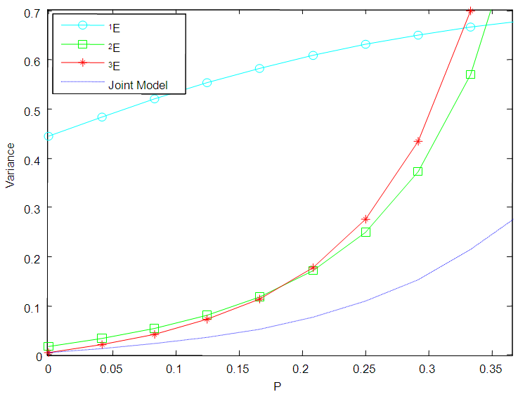
7. Comparison of Variances
In this section, the graphs of the variance of  of 1E-, 2E- and 3E-experiments and joint model for various values of
  and
and  versus
  are plotted for comparison purposes.It is observed from Figures 7 to 12 that:i)
  is smaller than
  and
and  for values of p close to 0, ii) for values of p close to 1 the
  is smaller than
  and
and  while iii) for some values of p between 0 and 1 the
  is smaller than the variance of the other two models. It is also noted that holding sensitivity and specificity constant and increasing the value of k from 2 to 10, makes the area in which the
  is smaller than the variance of the other models shrinks. Increasing sensitivity and specificity of the tests shrinks the area between
  and
and  It is also observed from Figures 7 to 12 that the variance of the joint model
 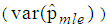 is smaller than the variance of p of the 1E-, 2E- and 3E-models. Hence the joint model is more reliable compared to the other three models.
 | Figure 7. A graph of  as a function of as a function of  with with  and and  |
 | Figure 8. A graph of  as a function of as a function of  with with 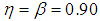 and and  |
 | Figure 9. A graph of  as a function of as a function of  with with  and and  |
 | Figure 10. A graph of  as a function of as a function of  with with  and and  |
 | Figure 11. A graph of  as a function of as a function of  with with  and and  |
 | Figure 12. A graph of  as a function of as a function of  with with  and and  |
8. Asymptotic Relative Efficiency (ARE)
The  and
and  are compared in this section. This is accomplished by computing asymptotic relative efficiency (ARE) values for various values of
  and
and  Let
Let
 and
and  From Tables 4 and 5 it is observed that increase in sensitivity and specificity of test leads to increase in the values of ARE. For the given values of pool size, sensitivity and specificity the highest value of ARE is 0.761. Hence the other models under consideration in the study 1E-, 2E- and 3E-models can only be 76.1% efficiency as the joint model.
 Table 4. The ARE of the joint model relative to the 1E-, 2E- and 3E-models with
 and and
 |
| |
|
Table 5. The ARE of the joint model relative to the 1E-, 2E- and 3E -models with

 |
| |
|
9. Conclusions
This study focused on construction of the a new model for approximating the prevalence rate of a trait in a population with imperfect tests by consecutively choosing between three experiments namely 1E-, 2E- and 3E -experiments. The model should select the better experiment and once the better experiment is being used, the estimator should approximate the individual maximum likelihood estimator (MLE) for that experiment. From this study it is clear that the best estimators for small, medium and large values of p, respectively, are  and
and  From Tables 2 and 3, the computed values of asymptotic relative efficiency (ARE) for various values of
  and
and  are less than one hence the proposed joint model for sequential choice of the best experiment for optimal estimation of a trait with misclassification is more efficient than the 1E-, 2E- and 3E-models.It is assumed that the samples being pooled for use in the model are independent and identically distributed Bernoulli random variables. It is also assumed that there is a laboratory test that can determine whether or not a unit or at least a unit in a pool has the characteristic of interest and that the tests are conditionally independent of each other. Sensitivity and specificity of the test kits are also assumed to be the same at each step of testing and for all samples in use in the model.The findings of the study of a better approximation of the prevalence rate have important health implications for prevention, intervention and treatment of HIV infections in a population. HIV infected population are known to greatly increase the spread of HIV infection. Our improved estimate of the prevalence rate of HIV infection could substantially reduce the potential risks for secondary HIV transmission by HIV infected population who are unaware of HIV infections. A prompt diagnosis of HIV infection might prevent the infected population from engaging in high-risk behaviours with uninfected population and avoid new HIV infections to occur. But the population with HIV infection should take counselling, regarding risk-reduction strategies such as abstinence and safer sexual behaviours such as 100% use of condoms. Based on the model developed a pool testing model of retesting of both positive and negative pools can be studied. A model based on cost analysis when sampling from different experiments can also be looked at when using imperfect kits.
Appendix
Appendix A: R code to Determine the Cut-Point Value of  and
and 
 Appendix B: R Code to Determine the Cut-Point Value of
  and
and 
 Appendix C: R Code to Determine the Cut-Point Value of
  and
and 
References
| [1] | Behets, F., Bertezzi, S., and Kasali, M., Kashamuka, M., Atikala, L., Brrown, C., Ryder, S., and Quinn, C., (1990). Successful use of Pooled Sera to Determine HIV-1 Seroprevalence in Zaire with Development of Cost-effective models. AIDS 4, 737-741. |
| [2] | Brookmeyer, R. (1999). Analysis of Multistage Pooling Studies of Biological Specimens for Estimating Disease Incidence and Prevalence. Biometric 55, 608 – 612. |
| [3] | Cahoon-Young, B., Chandler, A., Livermore, T., and Benjamir, R. (1989). Sensitivity and Specificity of Pooled versus Individual Sera in a Human Immunodeficiency Virus (HIV) antibody Prevalence Study. Journal of Clinical Microbiology 17, 1893-1895. |
| [4] | Ding, J. and Xiong, W. (2015). Robust Groups Testing for Multiple Traits with Misclassifications. Journal of Applied Statistics. Vol 42, no 10, 2115-2025. |
| [5] | Dorfman, R. (1943). The Detection of Defective Members of Large Population. Annals of Mathematical Statistics 14, 436-440. |
| [6] | Gastwirth, J. L., and Johnson, W. O. (1994). Screening with Cost-effective Quality Control: Estimation of Prevalence of a Rare Disease, Preserving the Anonymity of the Subject by Pool-testing; Application to Estimating the Prevalence of AIDS Antibodies in Blood Donors. Journal of statistical planning and inferences, 22, 15–27. |
| [7] | Hammick, P. A. and Gastwirth, J. L. (1994). Extending the Applicability of Estimation of Prevalence of Sensitive Characteristics by Pool Testing to Moderate Prevalence Populations. International Statistical Review 62, 319-331. |
| [8] | Hardwick, J., Connie, P. and Quentin, F. S. (1998). Sequentially Deciding Between Two Experiments for Estimating a Common Success Probability. Journal of the American statistical association. December 1998, vol 93 no 444, 1502-1511. |
| [9] | Kline, R. L., Bothus, T., Brookmeyer, R., Zeyer, S., and Quinn, T. (1989). Evaluation of Human Immunodeficiency Virus Seroprevalence in Population Surveys using Pooled Sera. Journal of clinical microbiology, 27, 1449-1452. |
| [10] | Maheswaran, S., Haragopal, V. V., and Pandit, S. N. N. (2008). Pool-testing using Block Testing Strategy. Journal of statistical planning and inference (Submitted). |
| [11] | Manzon, O. T., Palalin, F. J. E., Dimaal, E., Balis, A. M., Samson, C., and Mitchel, S. (1992). Relevance of Antibody Content and Test Format in HIV Testing of Pooled Sera. AIDS, 6, 43-48. |
| [12] | Nyongesa, L. K. (2011). Dual Estimation of Prevalence and Disease Incidence in Pool-Testing Strategy. Communication in Statistics Theory and Method, 40, 3218 - 3229. |
| [13] | Swallow, W. H. (1985). Group Testing for Estimating infection Rates and Probability of disease Transmissions. Phytopathology 75, 882-889. |
| [14] | Syaywa, J. P. and Nyongesa, L. K. (2010). Pool Testing with Test Errors Made Easier. International Journal of Computational Statistics. |
| [15] | Tamba, C. L., Nyongesa, K. L. Mwangi, J. W. (2012). Computational Pool-Testing Strategy. Egerton University Journal, 11:51-56. |
| [16] | Thomson, K. H. (1962). Estimation of the Population of Vectors in a Natural Population of Insects. Biometrics, 18, 568 - 578. |
| [17] | Tu, X. M., Litvak, E., and Pagano, M. (1995). On the Informativeness and Accuracy of Pooled Testing in Estimating Prevalence of a Rare Disease: Application to HIV Screening. Biometrika 82, 287-297. |
| [18] | Xie, M., Tatsuoka, K., Sacks, J and Young, S. (2001). Pool Testing with Blockers and Synergism. Journal of American Statistical Association 96, 92 - 102. |

 Abstract
 Reference
 Full-Text PDF
 Full-text HTML